“TensorBoard - Visualize your learning.”
TensorBoard
TensorBoard is a browser based application that helps you to visualize your training parameters (like weights & biases), metrics (like loss), hyper parameters or any statistics. For example, we plot the histogram distribution of the weight for the first fully connected layer every 20 iterations.
Namespace
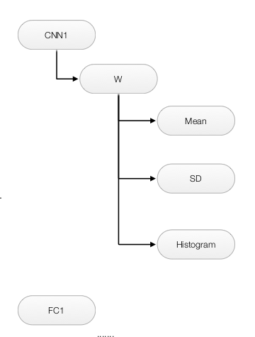
To create some data hierarchy structure when we view the data like:
We use namespace
with tf.name_scope('CNN1'):
    with tf.name_scope('W'):
        mean = tf.reduce_mean(W)
        tf.summary.scalar('mean', mean)
	stddev = tf.sqrt(tf.reduce_mean(tf.square(W - mean)))
	tf.summary.scalar('stddev', stddev)
        tf.summary.histogram('histogram', var)
Which create the following data hierarchy and can be browsed with the TensorBoard later:
Implement TensorBoard
To add & view data summaries to the TensorBoard. We need to:
- Define all the summary information to be logged.
- Add summary information to the writer to flush it out to a log file.
- View the data in the TensorBoard.
Define summary information
Number can be added to the TensorBoard with tf_summary.scalar and array with tf.summary.histogram
with tf.name_scope('CNN1'):
    with tf.name_scope('W'):
        mean = tf.reduce_mean(W)
        tf.summary.scalar('mean', mean)
        tf.summary.histogram('histogram', var)
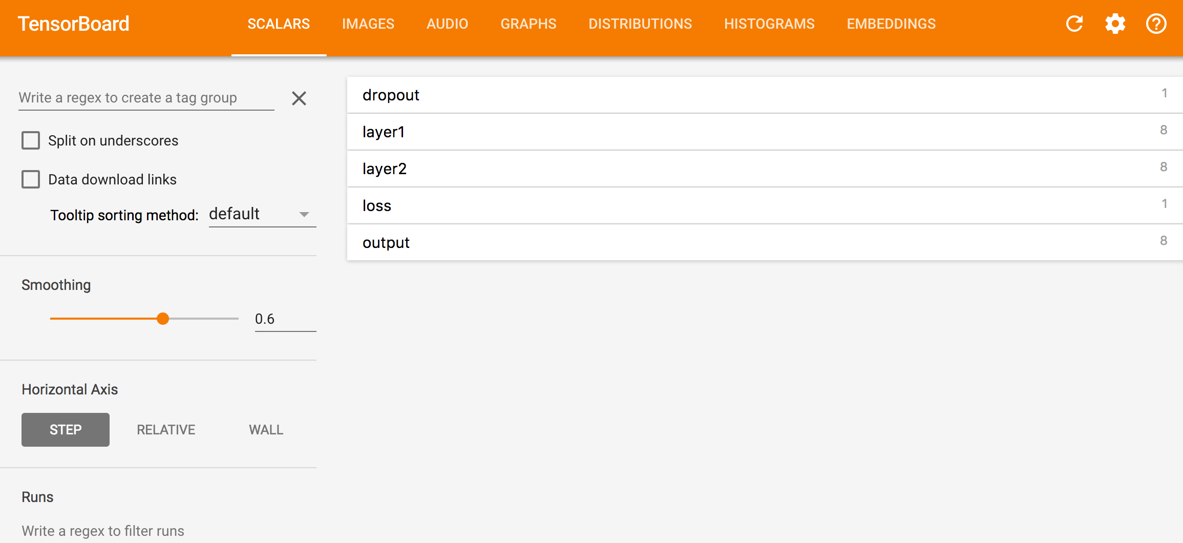
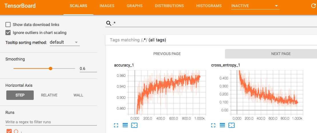
For data logged with tf_summary.scalar. The accuracy increases while cost drops.
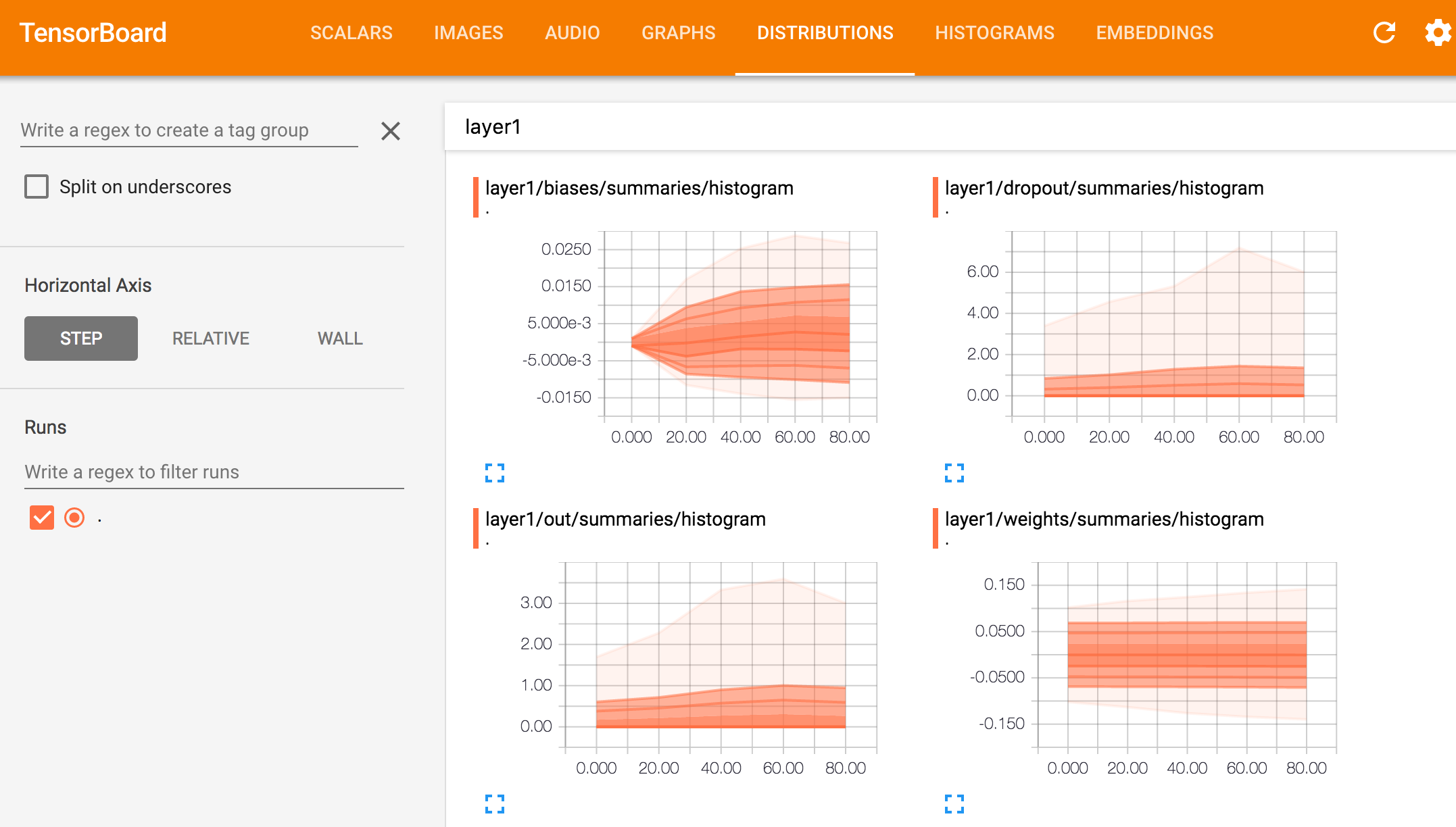
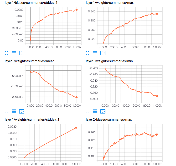
More statistics on the weights for layer 1.
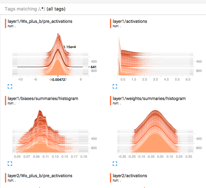
For summary logged with tf.summary.histogram
Example
Here is a more complicated example in which we try to summarize the information of the weight in the first fully connected layer.
h1, _ = affine_layer(x, 'layer1', [784, 256], keep_prob)
def affine_layer(x, name, shape, keep_prob, act_fn=tf.nn.relu):
    with tf.name_scope(name):
        with tf.name_scope('weights'):
            W = tf.Variable(tf.truncated_normal(shape, stddev=np.sqrt(2.0 / shape[0])))
            variable_summaries(W)
def variable_summaries(var):
  with tf.name_scope('summaries'):
    mean = tf.reduce_mean(var)
    tf.summary.scalar('mean', mean)
    with tf.name_scope('stddev'):
      stddev = tf.sqrt(tf.reduce_mean(tf.square(var - mean)))
    tf.summary.scalar('stddev', stddev)
    tf.summary.scalar('max', tf.reduce_max(var))
    tf.summary.scalar('min', tf.reduce_min(var))
    tf.summary.histogram('histogram', var)
Add summary information to a writer
After we define what summary information to be logged, we merge all the summary data into one single operation node with tf.summary.merge_all(). We create a summary writer with tf.summary.FileWriter, and then write and flush out the information to the log file every 20 iterations:
def main(_):
  ...
  train_step = tf.train.AdamOptimizer(learning_rate=0.001).minimize(cross_entropy)

  # Merge all summary inforation.
  summary = tf.summary.merge_all()

  init = tf.global_variables_initializer()
  with tf.Session() as sess:

      # Create a writer for the summary data.
      summary_writer = tf.summary.FileWriter(FLAGS.log_dir, sess.graph)

      sess.run(init)
      for step in range(100):
        ...
        sess.run(train_step, feed_dict={x: batch_xs, labels: batch_ys, lmbda:5e-5, keep_prob:0.5})
        if step % 20 == 0:
		 # Write summary
          summary_str = sess.run(summary, feed_dict={x: batch_xs, labels: batch_ys, lmbda:5e-5, keep_prob:0.5})
          summary_writer.add_summary(summary_str, step)
          summary_writer.flush()
        ...
Multimodal distributions
We can concatenate 2 Tensors to be plotted together in the same graph:
normal_combined = tf.concat([mean_moving_normal, variance_shrinking_normal], 0)
tf.summary.histogram("normal/bimodal", normal_combined)
Plot training and validation loss/accuracy
We use the same tensor to compute the loss for the training samples and validation samples. To plot the same tensor with different datasets together, Barzin provides a solution using 2 file writers:
import tensorflow as tf
from numpy import random

writer_1 = tf.summary.FileWriter("./logs/plot_1")
writer_2 = tf.summary.FileWriter("./logs/plot_2")

log_var = tf.Variable(0.0)
tf.summary.scalar("loss", log_var)

write_op = tf.summary.merge_all()

session = tf.InteractiveSession()
session.run(tf.global_variables_initializer())

for i in range(100):
    # for writer 1
    summary = session.run(write_op, {log_var: random.rand()})
    writer_1.add_summary(summary, i)
    writer_1.flush()

    # for writer 2
    summary = session.run(write_op, {log_var: random.rand()})
    writer_2.add_summary(summary, i)
    writer_2.flush()
View the TensorBoard
Open the terminal and run the Tensorboard command with you log file location.
$ tensorboard --logdir=/tmp/tensorflow/mnist/log
Starting TensorBoard b'41' on port 6006
(You can navigate to http://192.134.44.11:6006)
Runtime metadata
We can add runtime performance information into the TensorBoard
      merged = tf.summary.merge_all()
      ...

      run_options = tf.RunOptions(trace_level=tf.RunOptions.FULL_TRACE)
      run_metadata = tf.RunMetadata()
      summary, _ = sess.run([merged, train_step],
                              feed_dict=feed_dict(True),
                              options=run_options,
                              run_metadata=run_metadata)
      train_writer.add_run_metadata(run_metadata, 'step%03d' % i)
      train_writer.add_summary(summary, i)
Full program listing
# Copyright 2015 The TensorFlow Authors. All Rights Reserved.
#
# Licensed under the Apache License, Version 2.0 (the 'License');
# you may not use this file except in compliance with the License.
# You may obtain a copy of the License at
#
#     http://www.apache.org/licenses/LICENSE-2.0
#
# Unless required by applicable law or agreed to in writing, software
# distributed under the License is distributed on an 'AS IS' BASIS,
# WITHOUT WARRANTIES OR CONDITIONS OF ANY KIND, either express or implied.
# See the License for the specific language governing permissions and
# limitations under the License.
# ==============================================================================
"""A simple MNIST classifier which displays summaries in TensorBoard.
This is an unimpressive MNIST model, but it is a good example of using
tf.name_scope to make a graph legible in the TensorBoard graph explorer, and of
naming summary tags so that they are grouped meaningfully in TensorBoard.
It demonstrates the functionality of every TensorBoard dashboard.
"""
from __future__ import absolute_import
from __future__ import division
from __future__ import print_function

import argparse
import os
import sys
z
import tensorflow as tf

from tensorflow.examples.tutorials.mnist import input_data

FLAGS = None


def train():
  # Import data
  mnist = input_data.read_data_sets(FLAGS.data_dir,
                                    one_hot=True,
                                    fake_data=FLAGS.fake_data)

  sess = tf.InteractiveSession()
  # Create a multilayer model.

  # Input placeholders
  with tf.name_scope('input'):
    x = tf.placeholder(tf.float32, [None, 784], name='x-input')
    y_ = tf.placeholder(tf.float32, [None, 10], name='y-input')

  with tf.name_scope('input_reshape'):
    image_shaped_input = tf.reshape(x, [-1, 28, 28, 1])
    tf.summary.image('input', image_shaped_input, 10)

  # We can't initialize these variables to 0 - the network will get stuck.
  def weight_variable(shape):
    """Create a weight variable with appropriate initialization."""
    initial = tf.truncated_normal(shape, stddev=0.1)
    return tf.Variable(initial)

  def bias_variable(shape):
    """Create a bias variable with appropriate initialization."""
    initial = tf.constant(0.1, shape=shape)
    return tf.Variable(initial)

  def variable_summaries(var):
    """Attach a lot of summaries to a Tensor (for TensorBoard visualization)."""
    with tf.name_scope('summaries'):
      mean = tf.reduce_mean(var)
      tf.summary.scalar('mean', mean)
      with tf.name_scope('stddev'):
        stddev = tf.sqrt(tf.reduce_mean(tf.square(var - mean)))
      tf.summary.scalar('stddev', stddev)
      tf.summary.scalar('max', tf.reduce_max(var))
      tf.summary.scalar('min', tf.reduce_min(var))
      tf.summary.histogram('histogram', var)

  def nn_layer(input_tensor, input_dim, output_dim, layer_name, act=tf.nn.relu):
    """Reusable code for making a simple neural net layer.
    It does a matrix multiply, bias add, and then uses ReLU to nonlinearize.
    It also sets up name scoping so that the resultant graph is easy to read,
    and adds a number of summary ops.
    """
    # Adding a name scope ensures logical grouping of the layers in the graph.
    with tf.name_scope(layer_name):
      # This Variable will hold the state of the weights for the layer
      with tf.name_scope('weights'):
        weights = weight_variable([input_dim, output_dim])
        variable_summaries(weights)
      with tf.name_scope('biases'):
        biases = bias_variable([output_dim])
        variable_summaries(biases)
      with tf.name_scope('Wx_plus_b'):
        preactivate = tf.matmul(input_tensor, weights) + biases
        tf.summary.histogram('pre_activations', preactivate)
      activations = act(preactivate, name='activation')
      tf.summary.histogram('activations', activations)
      return activations

  hidden1 = nn_layer(x, 784, 500, 'layer1')

  with tf.name_scope('dropout'):
    keep_prob = tf.placeholder(tf.float32)
    tf.summary.scalar('dropout_keep_probability', keep_prob)
    dropped = tf.nn.dropout(hidden1, keep_prob)

  # Do not apply softmax activation yet, see below.
  y = nn_layer(dropped, 500, 10, 'layer2', act=tf.identity)

  with tf.name_scope('cross_entropy'):
    # The raw formulation of cross-entropy,
    #
    # tf.reduce_mean(-tf.reduce_sum(y_ * tf.log(tf.softmax(y)),
    #                               reduction_indices=[1]))
    #
    # can be numerically unstable.
    #
    # So here we use tf.nn.softmax_cross_entropy_with_logits on the
    # raw outputs of the nn_layer above, and then average across
    # the batch.
    diff = tf.nn.softmax_cross_entropy_with_logits(labels=y_, logits=y)
    with tf.name_scope('total'):
      cross_entropy = tf.reduce_mean(diff)
  tf.summary.scalar('cross_entropy', cross_entropy)

  with tf.name_scope('train'):
    train_step = tf.train.AdamOptimizer(FLAGS.learning_rate).minimize(
        cross_entropy)

  with tf.name_scope('accuracy'):
    with tf.name_scope('correct_prediction'):
      correct_prediction = tf.equal(tf.argmax(y, 1), tf.argmax(y_, 1))
    with tf.name_scope('accuracy'):
      accuracy = tf.reduce_mean(tf.cast(correct_prediction, tf.float32))
  tf.summary.scalar('accuracy', accuracy)

  # Merge all the summaries and write them out to
  # /tmp/tensorflow/mnist/logs/mnist_with_summaries (by default)
  merged = tf.summary.merge_all()
  train_writer = tf.summary.FileWriter(FLAGS.log_dir + '/train', sess.graph)
  test_writer = tf.summary.FileWriter(FLAGS.log_dir + '/test')
  tf.global_variables_initializer().run()

  # Train the model, and also write summaries.
  # Every 10th step, measure test-set accuracy, and write test summaries
  # All other steps, run train_step on training data, & add training summaries

  def feed_dict(train):
    """Make a TensorFlow feed_dict: maps data onto Tensor placeholders."""
    if train or FLAGS.fake_data:
      xs, ys = mnist.train.next_batch(100, fake_data=FLAGS.fake_data)
      k = FLAGS.dropout
    else:
      xs, ys = mnist.test.images, mnist.test.labels
      k = 1.0
    return {x: xs, y_: ys, keep_prob: k}

  for i in range(FLAGS.max_steps):
    if i % 10 == 0:  # Record summaries and test-set accuracy
      summary, acc = sess.run([merged, accuracy], feed_dict=feed_dict(False))
      test_writer.add_summary(summary, i)
      print('Accuracy at step %s: %s' % (i, acc))
    else:  # Record train set summaries, and train
      if i % 100 == 99:  # Record execution stats
        run_options = tf.RunOptions(trace_level=tf.RunOptions.FULL_TRACE)
        run_metadata = tf.RunMetadata()
        summary, _ = sess.run([merged, train_step],
                              feed_dict=feed_dict(True),
                              options=run_options,
                              run_metadata=run_metadata)
        train_writer.add_run_metadata(run_metadata, 'step%03d' % i)
        train_writer.add_summary(summary, i)
        print('Adding run metadata for', i)
      else:  # Record a summary
        summary, _ = sess.run([merged, train_step], feed_dict=feed_dict(True))
        train_writer.add_summary(summary, i)
  train_writer.close()
  test_writer.close()


def main(_):
  if tf.gfile.Exists(FLAGS.log_dir):
    tf.gfile.DeleteRecursively(FLAGS.log_dir)
  tf.gfile.MakeDirs(FLAGS.log_dir)
  train()


if __name__ == '__main__':
  parser = argparse.ArgumentParser()
  parser.add_argument('--fake_data', nargs='?', const=True, type=bool,
                      default=False,
                      help='If true, uses fake data for unit testing.')
  parser.add_argument('--max_steps', type=int, default=1000,
                      help='Number of steps to run trainer.')
  parser.add_argument('--learning_rate', type=float, default=0.001,
                      help='Initial learning rate')
  parser.add_argument('--dropout', type=float, default=0.9,
                      help='Keep probability for training dropout.')
  parser.add_argument(
      '--data_dir',
      type=str,
      default=os.path.join(os.getenv('TEST_TMPDIR', '/tmp'),
                           'tensorflow/mnist/input_data'),
      help='Directory for storing input data')
  parser.add_argument(
      '--log_dir',
      type=str,
      default=os.path.join(os.getenv('TEST_TMPDIR', '/tmp'),
                           'tensorflow/mnist/logs/mnist_with_summaries'),
      help='Summaries log directory')
  FLAGS, unparsed = parser.parse_known_args()
  tf.app.run(main=main, argv=[sys.argv[0]] + unparsed)

# 0.9816
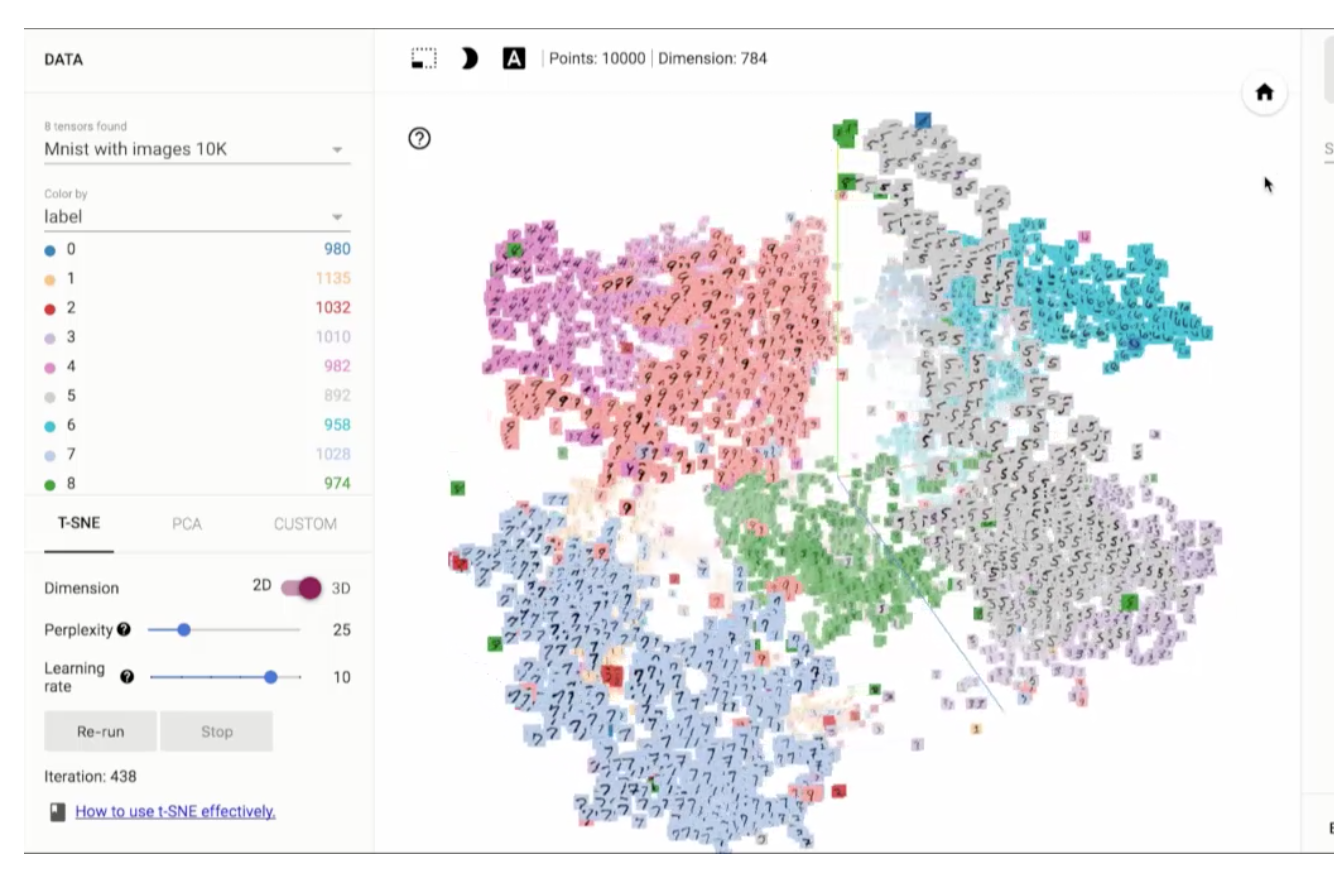
TensorBoard images & embedding
TensorFlow can also plot many different kinds of information including images and word embedding. To add image summary:
image = tf.reshape(x[:1], [-1, 28, 28, 1])
tf.summary.image("image", image)
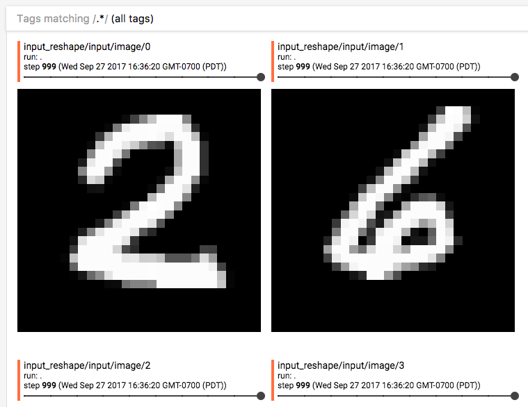
Image source from TensorFlow:
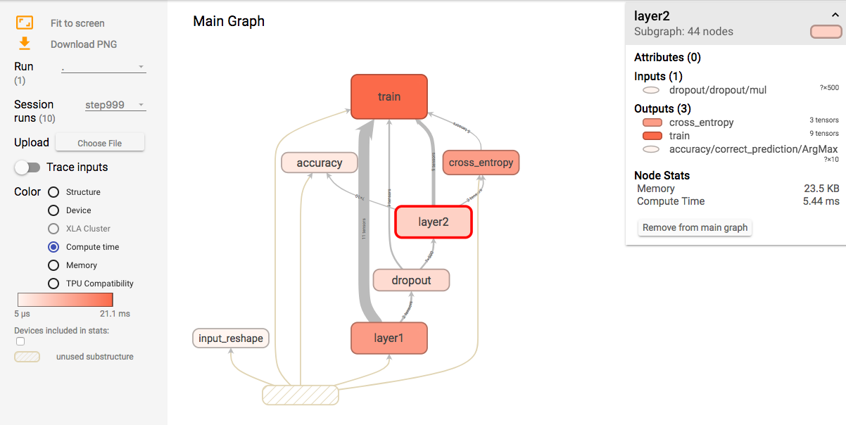
TensorBoard graph & distribution
TensorFlow automatically plots the computational graph and can be viewed under the graph tab.
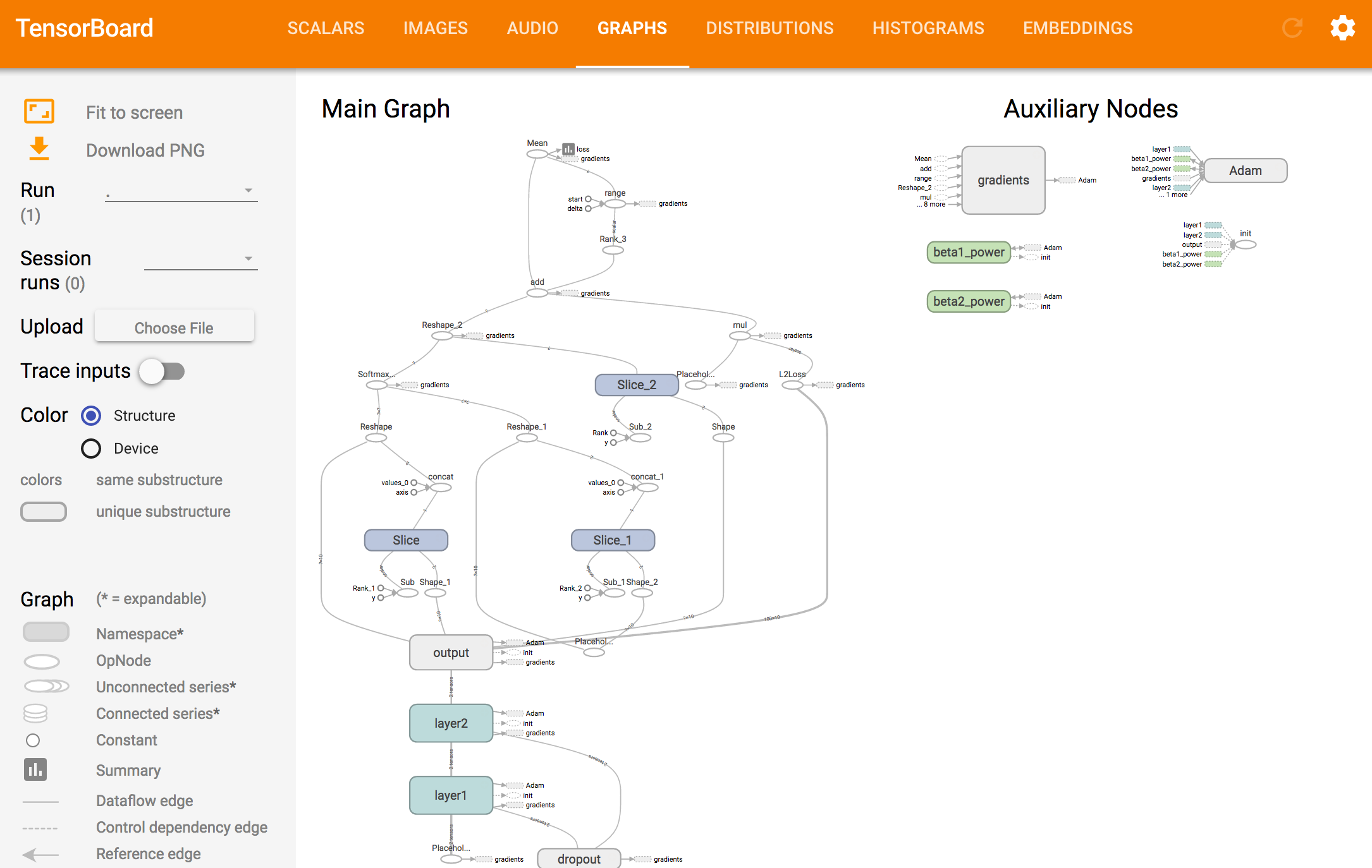
All histogram can also view as distribution.