“Deep learning - Information theory & Maximum likelihood.”
Information theory
Information theory quantifies the amount of information present. In information theory, the amount of information is characterized as:
- Predictability:
- Guaranteed events have zero information.
- Likely events have little information. (Biased dice have little information.)
- Random events process more information. (Random dice have more information.)
- Independent events add information. Rolling a dice twice with heads have twice the information of rolling the dice once with a head.
In information theory, chaos processes more information.
Information of an event is defined as:
\[I(x) = - \log(P(x))\]Entropy
In information theory, entropy measures the amount of information.
We define entropy as:
\[\begin{split} H(x) & = E_{x \sim P}[I(x)] \\ \end{split}\]So
\[\begin{split} H(x) & = − \mathbb{E}_{x \sim P} [log P(x)] \\ H(x) & = - \sum_x P(x) \log P(x) \\ \end{split}\]If \(\log\) has a base of 2, it measure the number of bits to encode the information. In information theory, information and random-ness are positively correlated. High entropy equals high randomness and requires more bits to encode it.
Example
Let’s comput the entropy of a coin. For a fair coin:
\[H(X) = - p(head) \cdot \log_2(p(head)) - p(tail) \cdot log_2(p(tail)) = - \log_2 \frac{1}{2} = 1\]Therefore we can use 1 bit to represent head (0 = head) and 1 bit to represent tail (1 = tail).
The entropy of a coin peaks when \(p(head)=p(tail)=0.5\).
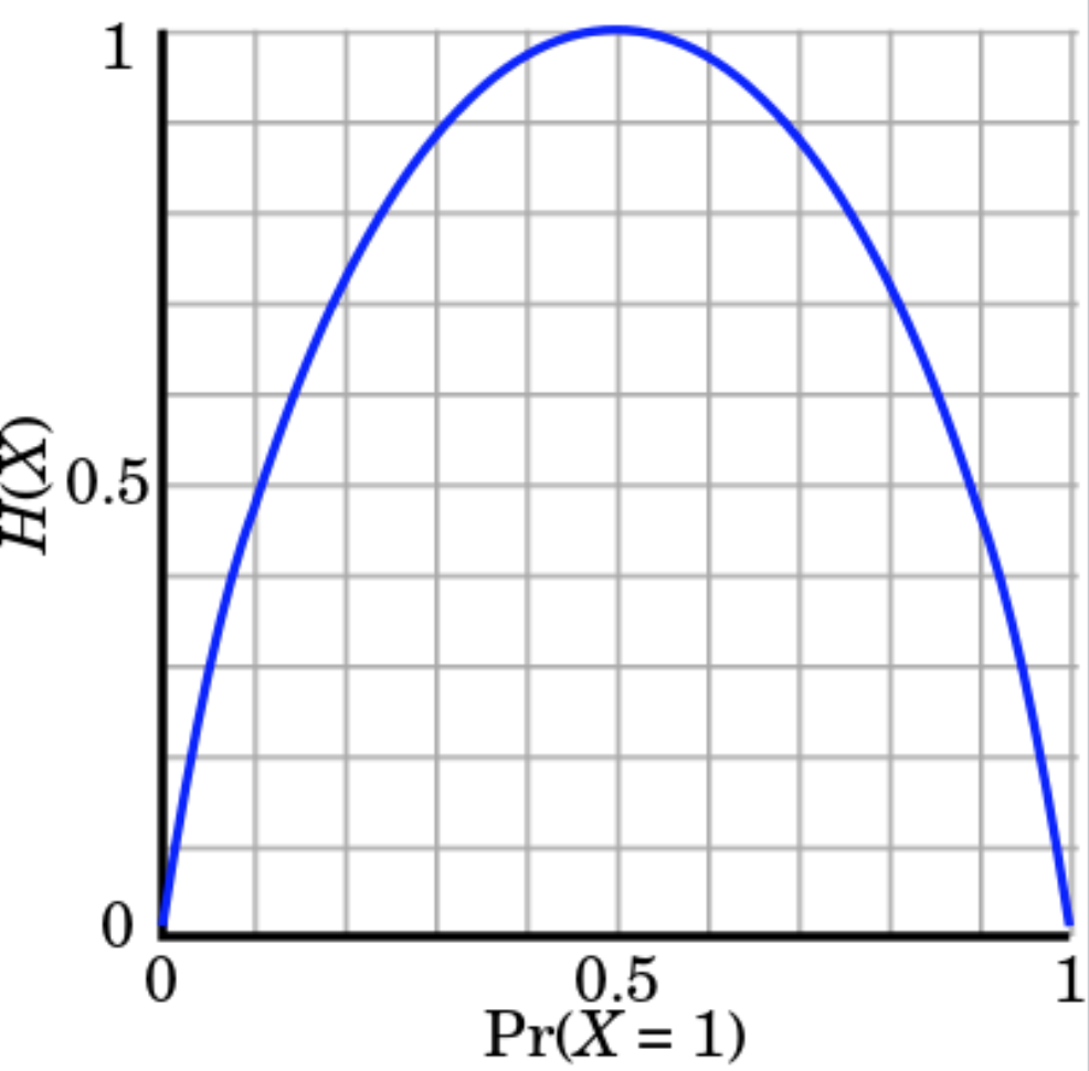
(Source Wikipedia)
For a fair die, \(H(X) = \log_2 6 \approx 2.59\). A fair die has more entropy than a fair coin because it is less predictable.
Cross entropy
If entropy measures the minimum number of bits to encode information, cross entropy measures the minimum of bits to encode \(x\) with distribution \(P\) using the wrong optimized encoding scheme from \(Q\).
Cross entropy is defined as:
\[H(P, Q) = - \sum_x P(x) \log Q(x)\]In deep learning, \(P\) is the distribution of the true labels, and \(Q\) is the probability distribution of the predictions from the deep network.
KL Divergence
In deep learning, we want a model predicting data distribution \(Q\) resemble the distribution \(P\) from the data. Such difference between 2 probability distributions can be measured by KL Divergence which is defined as:
\[\begin{split} D_{KL}(P \vert \vert Q) = \mathbb{E}_x \log \frac{P(x)}{Q(x)} \end{split}\]So,
\[\begin{split} D_{KL}(P \vert \vert Q) & = \sum_{x=1}^N P(x) \log \frac{P(x)}{Q(x)} \\ & = \sum_{x=1}^N P(x) [\log P(x) - \log Q(x)] \end{split}\]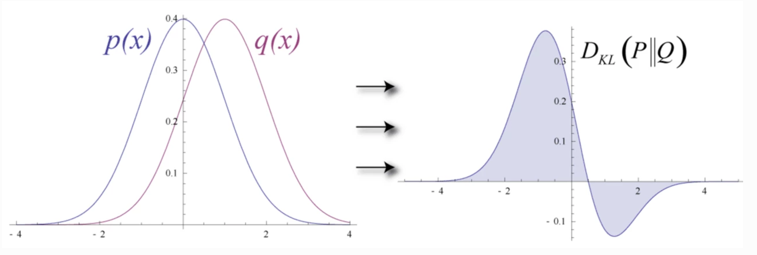
(Source Wikipedia.)
KL-divergence is not commutative: \(D_{KL}(P \vert \vert Q) \neq D_{KL}(Q \vert \vert P)\).
Recall:
\[\begin{split} H(P) & = - \sum P \log P, \\ H(P, Q) & = - \sum P \log Q, \quad \text{and}\\ D_{KL}(P \vert \vert Q) & = \sum P \log \frac{P}{Q}. \\ \end{split}\]We can rewrite the cross entropy equation with KL divergence:
\[\begin{split} H(P, Q) & = - \sum P \log Q \\ & = - \sum P \log P + \sum P \log P - \sum P \log Q \\ & = H(P) + \sum P \log \frac{P}{Q} \\ H(P, Q) & = H(P) + D_{KL}(P \vert \vert Q) \\ \end{split}\]So cross entropy is the sum of entropy and KL-divergence. Cross entropy \(H(P, Q)\) is larger than \(H(P)\) since we require extra amount of information (bits) to encode data with less optimized scheme from \(Q\) if \(P \neq Q\). Hence, KL-divergence is always positive for \(P \neq Q\) or zero otherwise.
\(H(P)\) only depends on \(P\): the probability distribution of the data. Since it is un-related with the model \(\theta\) we build, we can treat \(H(P)\) as a constant. Therefore, minimizing the cross entropy is equivalent to minimize the KL-divergence.
\[\begin{split} H(P, Q_\theta) & = H(P) + D_{KL}(P \vert \vert Q_\theta) \\ \nabla_\theta H(P, Q_\theta) & = \nabla_\theta ( H(P) + D_{KL}(P \vert \vert Q_\theta) ) \\ & = \nabla_\theta D_{KL}(P \vert \vert Q_\theta) \\ \end{split}\]Maximum Likelihood Estimation
We want to build a model with \(\hat\theta\) that maximizes the probability of the observed data (a model that fits the data the best: Maximum Likelihood Estimation MLE):
\[\begin{split} \hat\theta & = \arg\max_{\theta} \prod^N_{i=1} p(x_i \vert \theta ) \\ \end{split}\]However, multiplications overflow or underflow easily. Since \(\log(x)\) is monotonic, optimize \(log(f(x))\) is the same as optimize \(f(x)\). So instead of the MLE, we take the \(\log\) and minimize the negative log likelihood (NLL).
\[\begin{split} \hat\theta & = \arg\min_{\theta} - \sum^N_{i=1} \log p(x_i \vert \theta ) \\ \end{split}\]NLL and minimizing cross entropy is equivalent:
\[\begin{split} \hat\theta & = \arg\min_{\theta} - \sum^N_{i=1} \log q(x_i \vert \theta ) \\ & = \arg\min_{\theta} - \sum_{x \in X} p(x) \log q(x \vert \theta ) \\ & = \arg\min_{\theta} H(p, q) \\ \end{split}\]Putting it together
We want to build a model that fits our data the best. We start with the maximum likelihood estimation (MLE) which later change to negative log likelihood to avoid overflow or underflow. Mathematically, the negative log likelihood and the cross entropy have the same equation. KL divergence provides another perspective in optimizing a model. However, even they uses different formula, they both end up with the same solution.
Cross entropy is one common objective function in deep learning.
Mean square error (MSE)
In a regression problem, \(y = f(x; w)\). In real life, we are dealing with un-certainty and in-complete information. So we may model the problem as:
\[\hat{y} = f(x; θ) \\ y \sim \mathcal{N}(y;μ=\hat{y}, σ^2) \\ p(y | x; θ) = \frac{1}{\sigma\sqrt{2\pi}} \exp({\frac{-(y - \hat{y})^{2} } {2\sigma^{2}}}) \\\]with \(\sigma\) pre-defined by users:
The log likelihood becomes optimizing the mean square error:
\[\begin{split} J &= \sum^m_{i=1} \log p(y | x; θ) \\ & = \sum^m_{i=1} \log \frac{1}{\sigma\sqrt{2\pi}} \exp({\frac{-(y^{(i)} - \hat{y^{(i)}})^{2} } {2\sigma^{2}}}) \\ & = \sum^m_{i=1} - \log(\sigma\sqrt{2\pi}) - \log \exp({\frac{(y^{(i)} - \hat{y^{(i)}})^{2} } {2\sigma^{2}}}) \\ & = \sum^m_{i=1} - \log(\sigma) - \frac{1}{2} \log( 2\pi) - {\frac{(y^{(i)} - \hat{y^{(i)}})^{2} } {2\sigma^{2}}} \\ & = - m\log(\sigma) - \frac{m}{2} \log( 2\pi) - \sum^m_{i=1} {\frac{(y^{(i)} - \hat{y^{(i)}})^{2} } {2\sigma^{2}}} \\ & = - m\log(\sigma) - \frac{m}{2} \log( 2\pi) - \sum^m_{i=1} {\frac{ \| y^{(i)} - \hat{y^{(i)}} \|^{2} } {2\sigma^{2}}} \\ \nabla_θ J & = - \nabla_θ \sum^m_{i=1} {\frac{ \| y^{(i)} - \hat{y^{(i)}} \|^{2} } {2\sigma^{2}}} \\ \end{split}\]Many cost functions used in deep learning, including the MSE, can be derived from the MLE.
Maximum A Posteriori (MAP)
MLE maximizes \(p(y \vert x; θ)\).
\[\begin{split} θ^* = \arg\max_θ (P(y \vert x; θ)) & = \arg\max_w \prod^n_{i=1} P( y \vert x; θ)\\ \end{split}\]Alternative, we can find the most likely \(θ\) given \(y\):
\[θ^{*}_{MAP} = \arg \max_θ p(θ \vert y) = \arg \max_θ \log p(y \vert θ) + \log p(θ) \\\]Apply Bayes’ theorem:
\[\begin{split} θ_{MAP} & = \arg \max_θ p(θ \vert y) \\ & = \arg \max_θ \log p(y \vert θ) + \log p(θ) - \log p(y)\\ & = \arg \max_θ \log p(y \vert θ) + \log p(θ) \\ \end{split}\]To demonstrate the idea, we use a Gaussian distribution of \(\mu=0, \sigma^2 = \frac{1}{\lambda}\) as the our prior:
\[\begin{split} p(θ) & = \frac{1}{\sqrt{2 \pi \frac{1}{\lambda}}} e^{-\frac{(θ - 0)^{2}}{2\frac{1}{\lambda}} } \\ \log p(θ) & = - \log {\sqrt{2 \pi \frac{1}{\lambda}}} + \log e^{- \frac{\lambda}{2}θ^2} \\ & = C^{'} - \frac{\lambda}{2}θ^2 \\ - \sum^N_{j=1} \log p(θ) &= C + \frac{\lambda}{2} \| θ \|^2 \quad \text{ L-2 regularization} \end{split}\]Assume the likelihood is also gaussian distributed:
\[\begin{split} p(y^{(i)} \vert θ) & \propto e^{ - \frac{(\hat{y}^{(i)} - y^{(i)})^2}{2 \sigma^2} } \\ - \sum^N_{i=1} \log p(y^{(i)} \vert θ) & \propto \frac{1}{2 \sigma^2} \| \hat{y}^{(i)} - y^{(i)} \|^2 \\ \end{split}\]So for a Gaussian distribution prior and likelihood, the cost function is
\[\begin{split} J(θ) & = \sum^N_{i=1} - \log p(y^{(i)} \vert θ) - \log p(θ) \\ & = - \sum^N_{i=1} \log p(y^{(i)} | θ) - \sum^d_{j=1} \log p(θ) \\ &= \frac{1}{2 \sigma^2} \| \hat{y}^{(i)} - y^{(i)} \|^2 + \frac{\lambda}{2} \| θ \|^2 + constant \end{split}\]which is the same as the MSE with L2-regularization.
If the likeliness is computed from a logistic function, the corresponding cost function is:
\[\begin{split} p(y_i \vert x_i, w) & = \frac{1}{ 1 + e^{- y_i w^T x_i} } \\ J(w) & = - \sum^N_{i=1} \log p(y_i \vert x_i, w) - \sum^d_{j=1} \log p(w_j) - C \\ &= \sum^N_{i=1} \log(1 + e^{- y_i w^T x_i}) + \frac{\lambda}{2} \| w \|^2 + constant \end{split}\]Like, MLE, MAP provides a mechanism to derive the cost function. However, MAP can also model the uncertainty into the cost function which turns out to be the regularization factor used in deep learning.
Nash Equilibrium
In the game theory, the Nash Equilibrium is reached when no player will change its strategy after considering all possible strategy of opponents. i.e. in the Nash equilibrium, no one will change its decision even after we will all the player strategy to everyone. A game can have 0, 1 or multiple Nash Equilibria.
The Prisoner’s Dilemma
In the prisoner’s dilemma problem, police arrests 2 suspects but only have evidence to charge them for a lesser crime with 1 month jail time. But if one of them confess, the other party will receive a 12 months jail time and the one confess will be released. Yet, if both confess, both will receive a jail time of 6 months. The first value in each cell is what Mary will get in jail time for each decision combinations while the second value is what Peter will get.
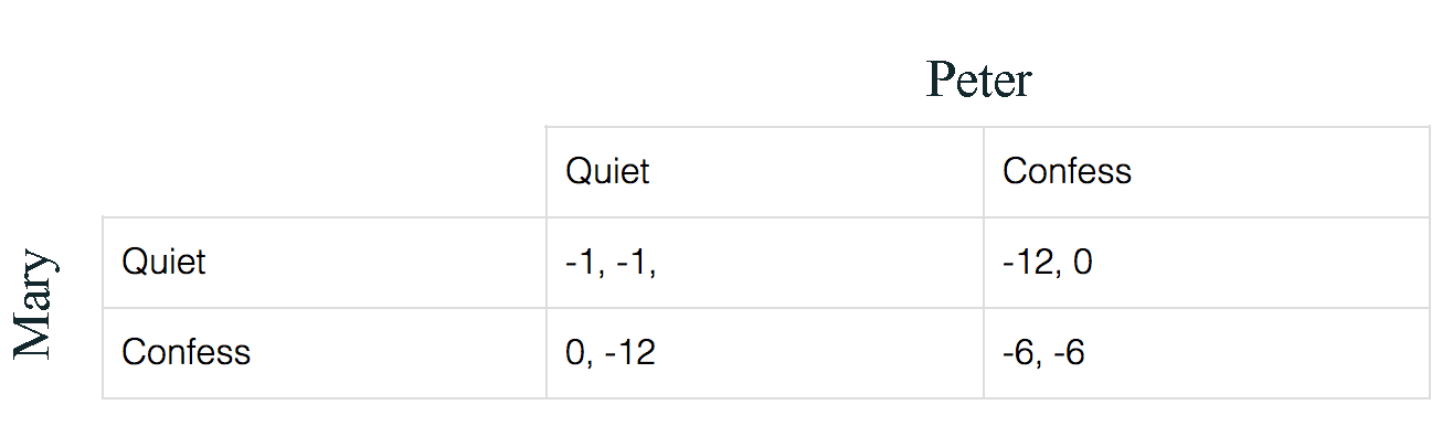
For Mary, if she thinks Peter will keep quiet, her best strategy will be confess to receive no jail time instead of 1 month.
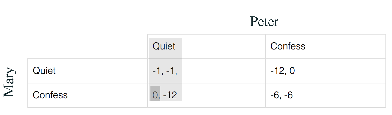
On the other hand, if she thinks Peter will confess, her best strategy will be confess also to get 6 months jail time.
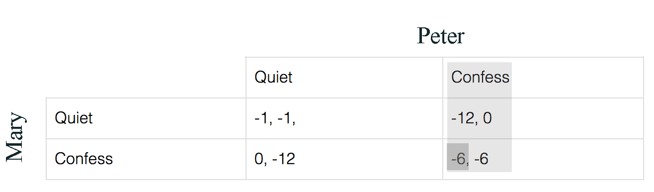
After knowing all possible actions, in either cases, Mary’s best action is to confess. Similarly, Peter should confess also. Therefore (-6, -6) is the Nash Equilibrium even (-1, -1) is the least jail time combined. Why (-1, -1) is not a Nash Equilibrium? Because if Mary knows Peter will keep quiet, she can switch to confess and get a lesser sentence which Peter will response by confessing the crime also. (Providing that Peter and Mary cannot co-ordinate their strategy.)
Jensen-Shannon Divergence
It measures how distinguishable two or more distributions are from each other.
\[JSD(X || Y) = H(\frac{X + Y}{2}) - \frac{H(X) + H(Y)}{2}\]