“Deep learning - Computation & optimization.”
Poor conditioning
Conditioning measures how rapidly the output changed with tiny changes in input.
For example, in a linear equation, we can use the inverse matrix \(A^{-1}\) to solve \(x\).
\[\begin{split} Ax & = b \\ x & = A^{-1} b \\ \end{split}\]Nevertheless it is not commonly done in machine learning because \(A^{-1}\) is slow to compute, and worse, \(A^{-1}\) may amplify input errors rapidly.
For the function:
\[f(b) = A^{-1}b \quad \text{where } A \in \mathbb{R}^{n \times n}.\]Condition number is defined as:
\[\underset{i, j}{\max} \left| \frac{\lambda_i}{\lambda_j} \right| \quad \text{where } \lambda_i, \lambda_j \text{ are the eigenvalues for } A.\]Poorly conditioned matrix \(A\) is a matrix with a high condition number. \(A^{-1}\) amplifies input errors. Small errors in \(x\) can change the output of \(A^{-1} x\) rapidly .
Other methods including matrix factorization can replace the matrix inversion method to avoid the poor conditioning to improve the numerical stability.
Underflow or overflow
Softmax functions:
\[softmax(x)_i = \frac{e^{x_i}}{\sum^n_{j=1} e^{x_j}}\]\(e^x\) can be very large or very small. To avoid overflow or underflow, we can transform \(x_j\) with \(\max(x)\):
\[\begin{split} m & = \max(x) \\ x_j & \rightarrow x_j - m = x^{'}_j\\ \end{split}\]Proof:
\[softmax(x)_i = \frac{e^{x_i}}{\sum e^{x_j}} = \frac{e^{-m} e^{x_i}}{e^{-m} \sum e^{x_j}} = \frac{e^{x_i - m}}{\sum e^{x_j - m}} = \frac{e^{x^{'}_i}}{\sum e^{x^{'}_j}}\]Jacobian matrix
\[f: \mathbb{R}^{n} \rightarrow \mathbb{R}^{m}\] \[J = \begin{pmatrix} \frac{\partial f_1}{ \partial x_1} & \frac{\partial f_1}{ \partial x_2} & \dots & \frac{\partial f_1}{ \partial x_n} \\ \frac{\partial f_2}{ \partial x_1} & \frac{\partial f_2}{ \partial x_2} & \dots & \frac{\partial f_2}{ \partial x_n} \\ \vdots & \vdots & \ddots & \vdots \\ \frac{\partial f_m}{ \partial x_1} & \frac{\partial f_m}{ \partial x_2} & \dots & \frac{\partial f_m}{ \partial x_n} \\ \end{pmatrix}\]Example:
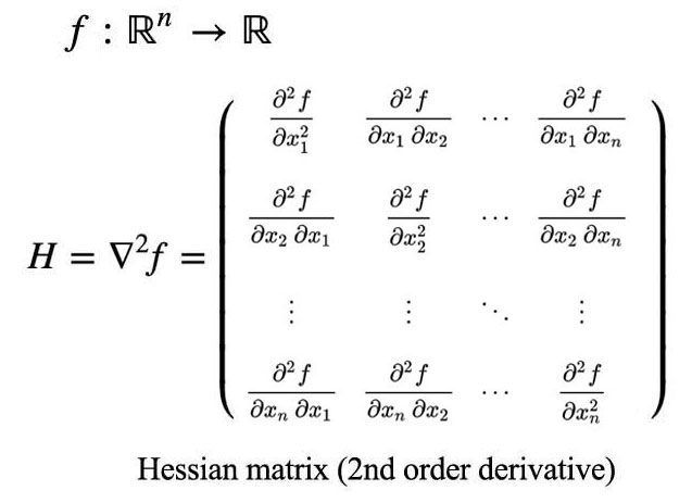
\[f: \mathbb{R}^{3} \rightarrow \mathbb{R}^{2} \\ f(x,y,z)=(xy+ y, 2xz) \\\] \[\begin{split} f_1 & = xy+ y \\ f_2 & = 2xyz \\ \end{split}\] \[\begin{split} \frac{\partial f_2}{ \partial x_2} &= \frac{\partial f_2}{ \partial y} = 2xz \\ \end{split}\]Hessian matrix
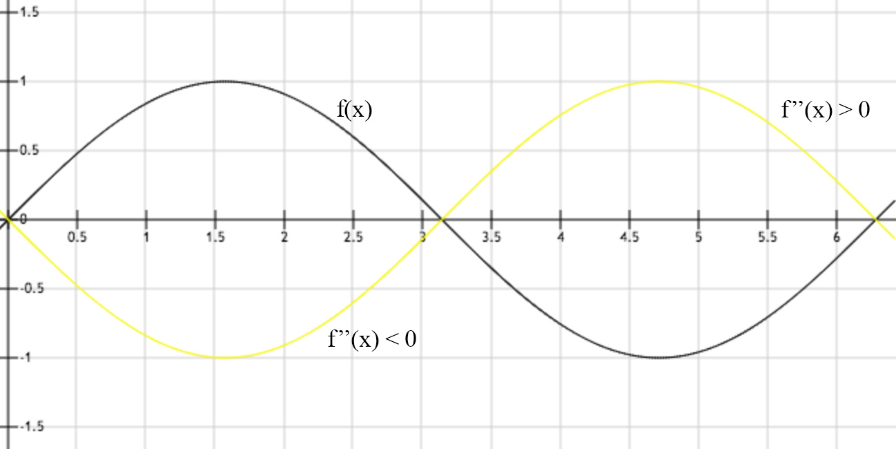
The first derivative measures the gradient and the second derivative measures the curvature.
When \(f''(x)<0\), \(f(x)\) curves down and when \(f''(x)>0\), \(f(x)\) curves up.
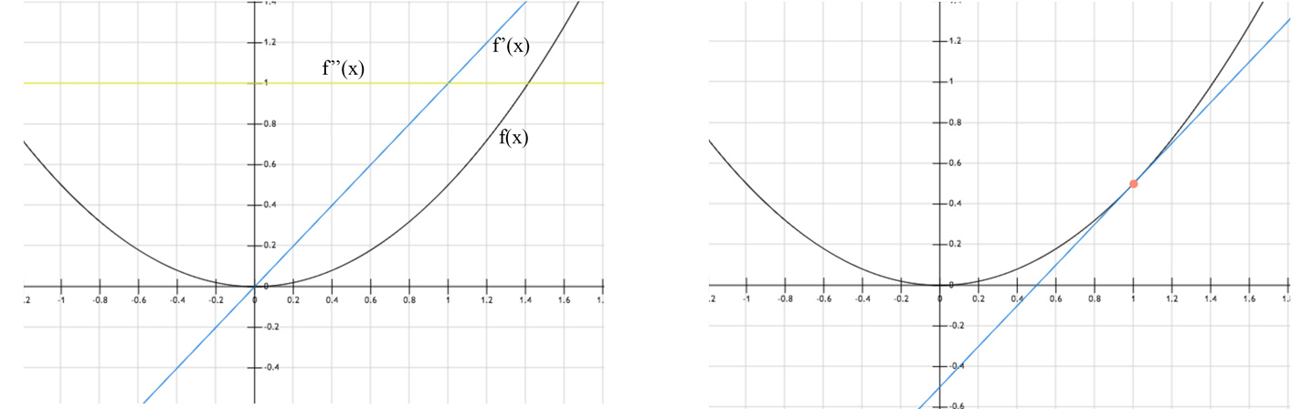
The second derivative indicates whether a gradient step drops the cost as much as the gradient alone may imply. For example, at \(x=1.0\) (the orange dot on the right below), the gradient is positive and the cost drops towards \(x=0\) direction. Since the second derivative is positive, the function curves upwards towards zero. i.e. the cost drops less than one predicted by the gradient alone.
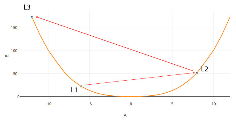
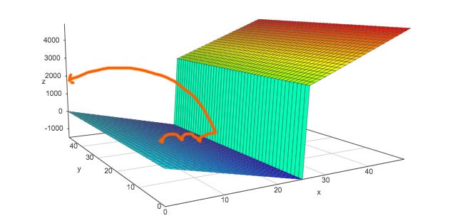
With the second derivative, we may take advantage of the curvature information to create a better gradient descent method to reduce overshoot. For example, instead of descending to a local minimum from \(L_1\), we may overshoot to \(L_2\) in the left diagram below. In some NLP problem, the gradient is so steep that we may bound upward to much higher cost.
Hessian matrix is defined as:
Eigenvalues for H
\(H\) is symmetrical:
\[\begin{split} & \frac{\delta^2}{\delta x_i \delta x_j} f(x) = \frac{\delta^2}{\delta x_j \delta x_i} f(x) \implies H_{ij} = H_{ji} \\ \end{split}\]And it is real. Any real symmetrical matrices can be decomposed into eigenvalues and eigenvectors. One more observation for the later use: the maximum value of \(g^T H g\) for vector \(v\) happens when \(v\) aligns with the eigenvector that has the maximum eigenvalue \(\lambda_{\max}\), i.e.
\[\begin{split} v^T H v & \leqslant v^T v \lambda_{\max} \\ \end{split}\]Learning rate
With Taylor series in 2nd order:
\[\begin{split} f(x) & = f(x^0) + (x-x^0)^T g + \frac{1}{2} (x-x^0)^T H (x-x^0) + \ldots \quad \text{where } g \text{ is the gradient.} \\ f(x) & \approx f(x^0) + (x-x^0)^T g + \frac{1}{2} (x-x^0)^T H (x-x^0) \\ f(x^0 - \epsilon g) & \approx f(x^0) - \epsilon g^T g + \frac{1}{2} \epsilon^2 g^T H g \\ \end{split}\]If \(g^T H g\) is negative or 0, \(f(x)\) decreases as \(ϵ\) increases. However, we cannot drop \(ϵ\) too far as the accuracy of the Taylor series drops as \(ϵ\) increases. If \(g^T H g\) is positive, it may cause \(f(x)\) to go up again. The optimal step for \(\epsilon\) is (assume \(\epsilon>0\)):
\[\begin{split} \epsilon^{*} & = \frac{g^T g}{g^T H g} \geqslant \frac{g^T g}{g^T g \lambda_{max}} = \frac{1}{\lambda_{max}} \quad \text{since } g^T H g \leqslant g^T g \lambda_{\max}.\\ \end{split}\]\(\lambda_{\max}\) is the maximum eigenvalue for \(H\). Hence, Hessian matrix \(H\) establishes a lower bound of the optimal learning rate.
\[\begin{split} f(x^{(0)} - \epsilon^{*} g) & \approx f(x^{(0)}) - \frac{1}{2} \epsilon^{*} g^T g \\ \end{split}\]If the Hessian matrix has a poor condition number, the gradient along the eigenvector with the largest eigenvalue \(\lambda_{\max}\) is much smaller than the one with the smallest eigenvalue. Gradient descent methods work poorly if the gradients in different directions are in different order of magnitude. The gradient descent methods will either learn too slow in the low gradient direction and/or overshoot the solution in the high gradient direction. We may use Newton’s method to control the gradient descent better.
Newton’s Method
With Newton’s method:
\[\begin{split} f(x) & \approx f(x^n) + f'(x^n)\Delta{x} + \frac{1}{2} f''(x^n)\Delta{x}^2 \\ \frac{ df(x)}{d\Delta{x}} & \approx f'(x^n)+ f''(x^n)\Delta{x} \\ \end{split}\]To find the critical point, we set \(\frac{ df(x)}{d\Delta{x}} =0\):
\[\begin{split} f'(x_n)+ f''(x_n)\Delta{x} = 0 \\ \Delta{x} = -\frac{f'(x_n)}{f''(x_n)} \\ \end{split}\]Apply:
\[\begin{split} x_{n+1} & = x_n + \Delta{x} \\ x_{n+1} & = x_n -\frac{f'(x_n)}{f''(x_n)} \\ \end{split}\]Extend it to multiple variables with \(H\):
\[\begin{split} x^{(n+1)} = x^{(n)} -[H f(x^{(n)})]^{-1} f'(x^{(n)})\\ \end{split}\]Apply the gradient descent with Newton’s method:
\[\begin{split} x^{'} = x - \epsilon [H f(x)]^{-1} f'(x) \\ \end{split}\]Saddle point
\(f'(x)=0\) alone cannot tell whether \(x\) is a local optimal point or a saddle point. With the second derivative test, when \(f'(x)=0\) and \(f''(x)>0\), \(x\) is a local minimum. When \(f'(x)=0\) and \(f''(x)<0\), \(x\) is a local maximum. However, if \(f''(x)=0\), it will be in-conclusive (saddle point or local optimal point).
For multiple dimension, when \(H\) is positive definite (all the eigenvalues are positive), \(x\) is a local minimum. If \(H\) is negative definite, \(x\) is a local maximum. If at least one eigenvalue is positive and at least one is negative, the point is a saddle point because one direction is a local minimum and the other direction is a local maximum. If at least one eigenvalue is zero and the rest have the same sign, it will be in-conclusive again.
Constrained Optimization
In deep learning, we may want to find an optimal point under certain constraints. For example, we want to maximize \(f(x, y)\) subject to \(g(x, y) = 0\). We will construct a new Lagrangian function \(\mathcal{L}(x, \lambda)\) from \(f\) and \(g\) which the original optimal solution is the same as the optimal solution for the Lagrangian function. i.e. \(\mathcal{L}^{'}(x, \lambda) = 0\).
Lagrange multiplier
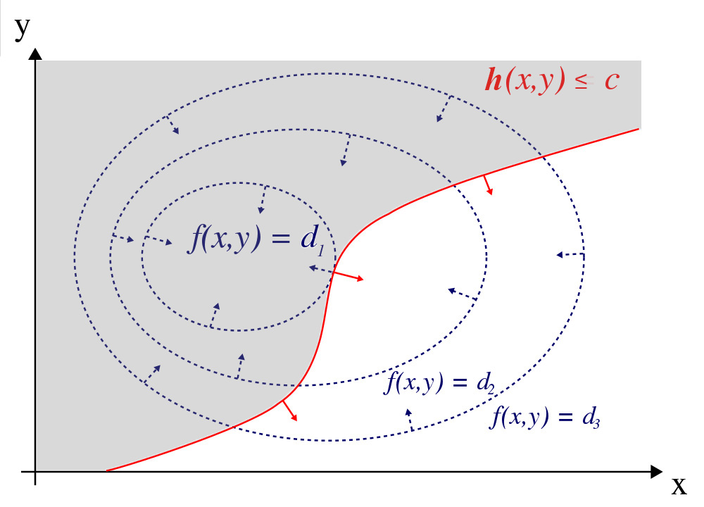
To maximize \(f(x, y)\) subject to \(g(x, y) = 0\), we plot the contour plot of \(f(x, y) = d_i\) for different \(d_i\) (\(d_1 > d_2 > d_3\)). The solution lies on the red line with the largest \(d_i\).
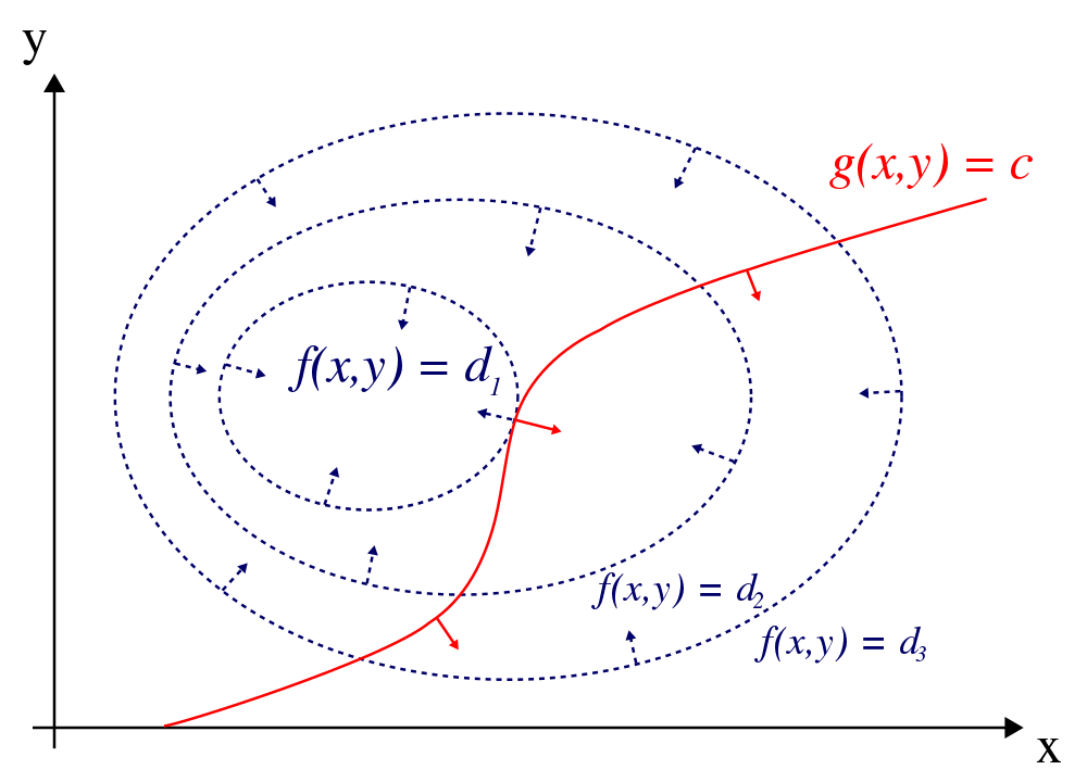
(Source Wikipedia)
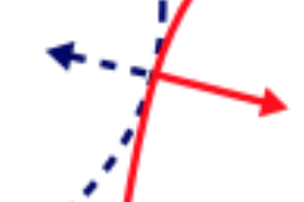
Geometrically, the optimal point lies where the gradient at \(f(x, y)\), the blue arrow, aligned with the gradient at \(g(x, y)\), the red arrow.
i.e.
\[\begin{split} \nabla_{x, y} f(x, y) = \lambda \nabla_{x, y} g(x, y) \\ \end{split}\]where \(\lambda\) is the Lagrange multiplier and it can be positive or negative. We can now solve a constrained optimization problem using unconstrained optimization of the generalized Lagrangian.
We can have multiple constraints (\(g^1, g^2 \ldots g^i\)). ie. we want to maximize \(f(x,y)\) subject to \(g^1(x,y)=0, \ldots, g^i(x,y)=0\). The Lagrangian is generalized as:
\[\mathcal{L} (x, \lambda) = f(x) + \sum_i \lambda_i g^{(i)}(x)\]And the optimal solution is
\[\mathcal{L}^{'} (x, \lambda) = 0\]Example
Maximize \(f\) subject to \(x^2 + y^2 = 32\)
\[\begin{split} f(x, y) = x + y \\ x^2 + y^2 - 32 = 0 \\ \end{split}\]The Lagrangian is:
\[\begin{split} \mathcal{L} (x, y, \lambda^{'}) = x + y + \lambda^{'} (x^2 + y^2 - 32) \text{ or}\\ \mathcal{L} (x, y, \lambda) = x + y + \lambda (0.5 x^2 +0.5 y^2 - 16) \\ \end{split}\]To optimize \(\mathcal{L}\), we need to solve:
\[\begin{split} \frac{\partial \mathcal{L}}{\partial x} &= 1 + \lambda x = 0 \implies x = \frac{-1}{\lambda}\\ \frac{\partial \mathcal{L}}{\partial y} &= 1 + \lambda y = 0 \implies y = \frac{-1}{\lambda}\\ \frac{\partial \mathcal{L}}{\partial \lambda} &= 0.5 x^2 + 0.5 y^2 - 16 = 0 \implies x^2 + y^2 = 32\\ \end{split}\]Therefore:
\[\begin{split} \lambda &= \pm \frac{1}{4} \\ x &= \pm 4 \\ y &= \pm 4 \\ \end{split}\]By simply plugin the values, we can determine which one is the max or min.
\[\begin{split} f(4, 4) = 8 = \max\\ f(-4, -4) = -8 = \min \\ \end{split}\]Karush–Kuhn–Tucker (KKT)
KKT expands the constraints in the Lagrange multiplier to inequality also:
\[\begin{split} & f(x, y) \quad \text{subject to } \\ & g^{i}(x, y) = 0 \\ & h^{i}(x, y) \leqslant 0 \\ \end{split}\]The Lagrangian is generalized to:
\[\mathcal{L} (x, \lambda, \alpha) = f(x) + \sum_i \lambda_i g^{(i)}(x) + \sum_j \alpha_j h^{(j)}(x)\]or
\[\underset{x}{\min} \underset{\lambda}{\max} \underset{\alpha, \alpha ≥ 0}{\max} \mathcal{L} (x, \lambda, \alpha)\]KKT conditions
The required KKT conditions to solve the optimization problems are:
\[\begin{split} \mathcal{L}^{'} (x, \lambda, \alpha) = 0 \\ \alpha_j \geqslant 0 \\ \alpha \cdot h(x^{*})=0 \\ \end{split}\]and the solution needs to be verified with the constraints again.
\[\begin{split} & g^{i}(x, y) = 0 \\ & h^{i}(x, y) \leqslant 0 \\ \end{split}\]Let’s go through the meaning of each KKT conditions. Same as Lagrange multiplier, the optimal points happen when the derivative \(\mathcal{L}^{'}=0\), i.e.
\[\begin{split} \mathcal{L}^{'} (x, \lambda, \alpha) = 0 \end{split}\]In the Lagrange multiplier, \(\lambda\) can be positive, negative or zero. In KKT. \(\alpha\) must be greater or equal to 0. This guarantees the in-equality such that the solution is within the constrained area.
\[\alpha_j \geqslant 0\]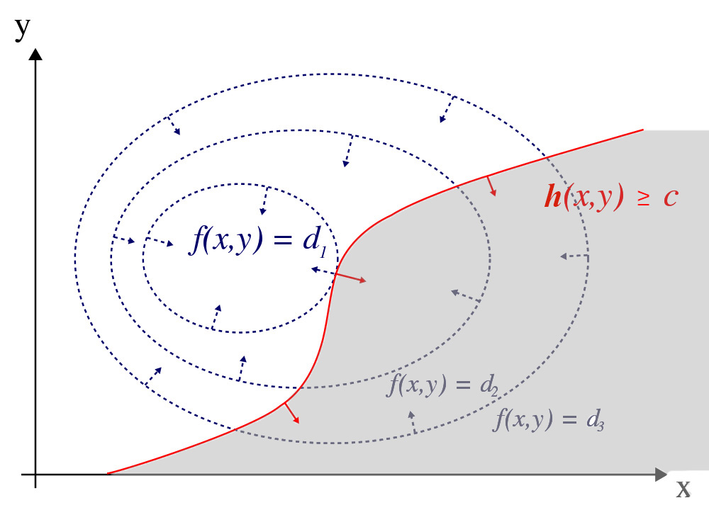
For
\[\alpha \cdot h(x^{*})=0,\]it indicates either the KKT multiplier \(\alpha_i=0\) or the \(h(x^{∗})=0\). If \(\alpha_i=0\), we do not care about the constraint. The in-equality constrain is not necessary like the diagram below because the optimal point is guarantee to be inside the constrained area. We can simply ignore the constraint.
Otherwise, the in-equality constrain becomes the equality constraint \(h(x^{*})=0\).
Terms
Line search
\[f(x - \epsilon \nabla_{x} f(x) )\]We sample the outputs of a few small \(\epsilon\) values and select \(x \rightarrow x - \epsilon \nabla_{x} f(x)\) that output the best optimal value.