“Deep learning - Probability & distribution.”
Probability mass function & probability density function
Probability mass function is the probability distribution for discret variables, for example, the probability of rolling a fair die with a value 2 is \(P(\mathrm{x} = 2) = \frac{1}{6}\)
It has an upper case notation \(P(\mathrm{x} = x)\). The plan text form \(\mathrm{x}\) represents the variable and the script form \(x\) represents the variable’s value. We use the bold form \(P(\boldsymbol{\mathrm{x}} = \boldsymbol{x})\) if \(\boldsymbol{\mathrm{x}}\) is a vector. We often shorten both notations to \(P(x)\) and \(P(\boldsymbol{x})\) for vector which include the variable’s values only. \(x \sim P(x)\) means sampling from the probability distribution of \(\mathrm{x}\).
Probability density function (PDF) is the probability distribution for continuous variables using lower case notation \(p(x)\). For example, the probability of completing a task between \(t\) and \(t+1\) seconds. Sum of all possibilities is equal to 1.
\[\int p(x)dx = 1\]\(\mathrm{x}\) is called a random variable whose values are the outcome of a random process, like rolling a dice five times. For example, \(P(\mathrm{x} = 15)\) holds the probability for \(\mathrm{x} = 15\) after five rolls.
Conditional probability
\[\begin{split} P(A \vert B) &= \frac{P(A, B)}{P(B)} \\ P(A, B) &= P(A \vert B) P(B) \\ \end{split}\]Apply last equation:
\[\begin{split} P(A, B \vert C) &= P(A \vert B, C) P(B \vert C) \\ \end{split}\]Chain rule
\[\begin{split} P (x^1, . . . , x^n) &= \bigg( \prod^{n-1}_{i=1} P (x^i | x^{i+1}, . . . , x^{n}) \bigg) P (x^n) \\ P (a, b, c, d) &= P(a | b, c, d) P(b, c, d) \\ & = P (a \vert b, c, d)P (b \vert c, d) P (c \vert d)P (d) \\ \end{split}\]Marginal probability
Marginal probability is the probability of a sub-set of variables. It is often calculated by summing over all the possibilities of other variables. For an example, with a discret variable \(\mathrm{x}\), we sum over all possibility of \(\mathrm{y}\):
\[P(x) = \sum_y P(x, y) = \sum_y P(x | y) P(y)\]or for continuous variables
\[p(x) = \int p(x, y)dy\]Independence
Given 2 events \(x_i, x_j\) are independent:
\[\begin{align} P(x_i, x_j ) & = P(x_i) P(x_j ) \\ P(x_i, x_j \vert y) & = P(x_i \vert y) P(x_j \vert y) \\ \end{align}\]Bayes’ theorem
\[\begin{split} P(A \vert B) & = \frac{P(B \vert A) P(A)}{P(B)} \\ P(A \vert B) & = \frac{P(B \vert A) P(A)}{\sum^n_i P(B, A_i) } = \frac{P(B \vert A) P(A)}{\sum^n_i P(B, \vert A_i) P(A_i) } \end{split}\]Apply Bayes’ theorem:
\[P(A \vert B, C) = \frac{P(B \vert A, C) P(A \vert C)}{ P(B \vert C)} \quad \text{a.k.a. apply Bayes to } P(A \vert B) \text{ first, then given C.}\]Terminology
In Bayes’ theorem,
\[\begin{split} P(H \vert E) & = \frac{P(E \vert H) \cdot P(H)}{P(E)} \\ \text{posterior} & = \frac{\text{likelihood } \cdot \text{prior}}{\text{marginal probability}} \\ \end{split}\]\(P(H)\) is called prior which quantifies our belief \(H\). We all start learning probability using a frequentist approach: we calculate the probability by \(\frac{\text{number of events}}{\text{total trials}}\). For a fair die, the chance of getting a tail \(P_t(tail)\) is 0.5. But if the total trials are small, the calculated value is unlikely accurate. In Bayes inference, we quantify all possibilities of getting a tail \(P(H)\) to deal with uncertainty. We want to find the probability of all the probabilities:
\[P(H=v) \quad \text{for all } v \in [0, 1]\]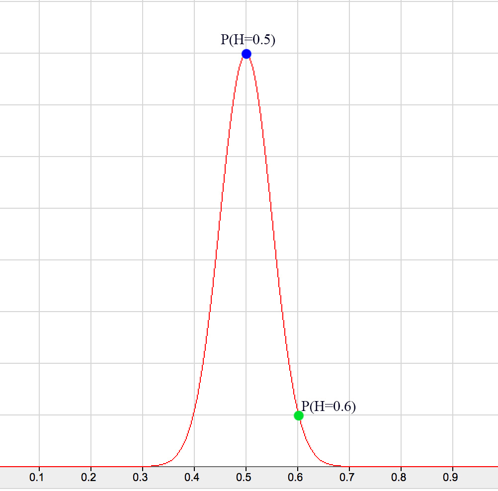
For example, \(P(H=0.6)\) means what is the probability of finding the coin has a 0.6 chance of getting a tail. Of course, it is much lower than \(P(H=0.5)\) if the coin is fair. We can use previous knowledge (including previous data) or assumption to define the prior at the beginning and re-adjust it with Bayes’ theorem with observed evidence. \(P(E \vert H)\) is the likelihood of the observed data \(E\) given the belief. (say, the likelihood of observing 2 tails in the next 2 trails) For example, if \(H=0.6\), the likelihood of seeing 2 tails are \(0.6 \times 0.6\). The posterior \(P(H \vert E)\) is the updated belief using Bayes’ equation above after taking the observed data into account. Since we see more tails in our evidence, the peak of the posterior is shifted to the right but not to \(H=1.0\) as the frequentist approach may calculate. As suspected, we are dealing with a series of probabilities rather than one single value. However, with the beta function, this can be done easily.
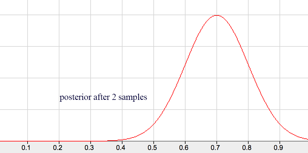
When the next round of sample data is available, we can apply the Bayes’ theorem again with the prior replaced by the last posterior. Bayes’ theorem works better than simple frequency calculation in particular the sampling error can be high when sampling size is small at the beginning.
As indicated by the naming, the observed data \(E\) is also called evidence and the belief \(H\) is also called hypothesis.
Bayes theorem can handle multiple variables \(P(A \vert B, C, D)\) and provide a better mathematical foundations than the frequentist approach.This section introduces the key terminology. In the later section on beta function, we will detail the implementation and the advantage.
Naive Bayes’ theorem
Naive Bayes’ theorem assume \(x_i\) and \(x_j\) are independent. i.e. \(\begin{align} P(x_i, x_j \vert y) & = P(x_i \vert y) P(x_j \vert y) \\ \end{align}\)
\[\begin{split} P(y \vert x_1, x_2, \cdots , x_n) & = \frac{P(x_1, x_2, \cdots , x_n \vert y) P(y)}{P(x_1, x_2, \cdots , x_n)} \\ & = \frac{P(x_1 \vert y) P(x_2 \vert y) \cdots P(x_n \vert y) P(y)}{P(x_1, x_2, \cdots , x_n)} \\ & \propto P(x_1 \vert y) P(x_2 \vert y) \cdots P(x_n \vert y) P(y) \\ \end{split}\]We often ignore the marginal property (the denominator) in Naive Bayes theorem because it is a constant. The probability of the evidence is un-related with \(y\). We usually compare calculated values rather than finding the absolute values. In particular, \(P(x_1, x_2, \cdots , x_n)\) may be too hard to find in some problems.
In detecting e-mail spam, \(y\) indicates whether the email is a spam. \(x_i\) represents the presence of the word \(i\) in our vocabulary. \(P(x_i \vert y)\) represents the chance that word \(i\) presence in a spam. We can collect the spam emails marked by users and calculate this probability easily. By trial and error, we can set a threshold for the calculated value before we mark it as a spam.
Expectation
The definition of expectation for discret variables:
\[\mathbb{E}_{x \sim P} [f(x)] = \sum_x P(x)f(x)\]Can be shorten as:
\[\mathbb{E}_{x} [f(x)]\]For continuous variables:
\[\mathbb{E}_{x \sim P} [f(x)] = \int p(x)f(x)dx\]Properties:
\[\mathbb{E}_{x} [\alpha f(x) + \beta g(x)] = \alpha \mathbb{E}_{x} [f(x)] + \beta \mathbb{E}_{x} [g(x)]\]Variance and covariance
\[\begin{split} Var(f(x)) & = \mathbb{E} [(f(x) − \mathbb{E}[f(x)])^2] \\ Cov(f(x), g(y)) & = \mathbb{E} \Big[\big(f(x) − \mathbb{E} [f(x)]\big) \big( g(y) − \mathbb{E} [g(y)] \big)\Big] \\ Cov(x_i, x_i) & = Var(x_i) \\ \end{split}\]Covariance measures how variables are related. If covariance is high, data tend to take on relatively high (or low) values simultaneously. If they are negative, the tends to take the opposite values simultaneously. If it is zero, they are linearly independent.
Gaussian distribution/Normal distribution
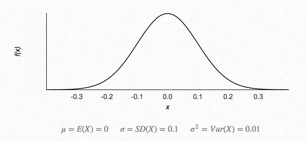
\(\mathcal{N}{\left(\mu=0 ,\sigma^2=1 \right)}\) is called standard normal distribution.
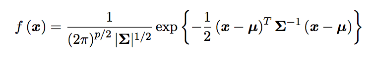
The PDF of a multivariate Gaussian distribution is defined as:
Bernoulli distributions
Source Wikipedia
\[\begin{split} P(\mathrm{x}=1) &= \phi \\ P(\mathrm{x}=0) &= 1 - \phi \\ \mathbb{E}_x[x] & = \phi \\ Var_x (x) & = \phi (1 - \phi) \\ \end{split}\]Binomial distributions
\[P(x;p,n) = \left( \begin{array}{c} n \\ x \end{array} \right) p^{x}(1 - p)^{n-x}\]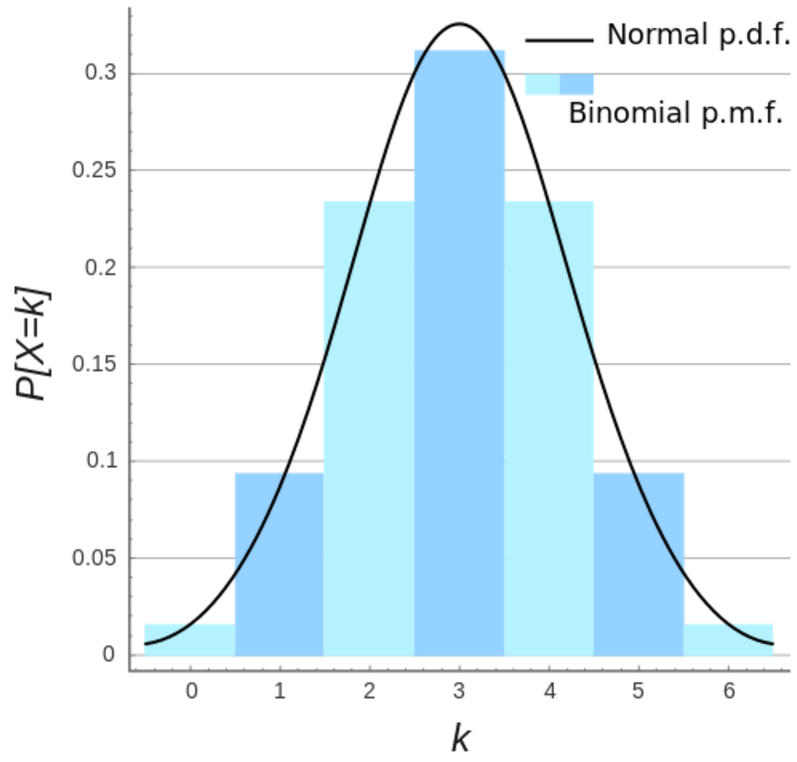
Source Wikipedia
The Gaussian distribution is the limiting case for the binomial distribution with:
\[\begin{split} \mu & = n p \\ \sigma^2 & = n p (1-p) \end{split}\]Poisson Distribution
Assuming a rare event with an event rate \(\lambda\), the probability of observing x events within an interval \(t\) is:
\[P(x) = \frac{e^{-\lambda t} (\lambda t)^x}{x!}\]Example: If there were 2 earthquakes per 10 years, what is the chance of having 3 earth quakes in 20 years.
\[\begin{split} \lambda t & = 2 \cdot (\frac{20}{10}) = 4 \\ P(x) & = \frac{e^{-\lambda t} (\lambda t)^x}{x!} \\ P(3) & = \frac{e^{-4} \cdot 4^3}{3!} \end{split}\]Given:
\[\begin{split} prob. & = p = \frac{v}{N} \\ P(x \vert N, p) & = \frac{N!}{x! (N-x)!} p^x(1-p)^{N-x} \\ \end{split}\]Proof:
\[\begin{split} P(x \vert v) & = \lim_{N\to\infty} P(x|N, v) \\ &= \lim_{N\to\infty} \frac{N!}{x! (N-x)!} (\frac{v}{N})^x(1-\frac{v}{N})^{N-x} \\ &= \lim_{N\to\infty} \frac{N(N-1)\cdots(N-x+1)}{N^x} \frac{v^x}{x!}(1-\frac{v}{N})^N(1-\frac{v}{N})^{-x} \\ &= 1 \cdot \frac{v^x}{x!} \cdot e^{-v} \cdot 1 & \text{Given } v \ll N \\ &= \frac{e^{-v} v^x }{x!} \\ &= \frac{e^{-\lambda t} (\lambda t)^x }{x!} & \text{Given } v = \lambda t \\\\ \end{split}\]Beta distribution
The definition of a beta distribution is:
\[\begin{align} P(\theta \vert a, b) = \frac{\theta^{a-1} (1-\theta)^{b-1}} {B(a, b)} \end{align}\]where \(a\) and \(b\) are parameters for the beta distribution.
For discret variable, the beta function \(B\) is defined as:
\[\begin{align} B(a, b) & = \frac{\Gamma(a) \Gamma(b)} {\Gamma(a + b)} \\ \Gamma(a) & = (a-1)! \end{align}\]For continuos variable, the beta function is:
\[\begin{align} B(a, b) = \int^1_0 \theta^{a-1} (1-\theta)^{b-1} d\theta \end{align}\]For our discussion, let \(\theta\) be the infection rate of the flu. With Bayes’ theorem, we study the probabilities of different infection rates rather than just finding the most likely infection rate. The prior \(P(\theta)\) is the belief on the probabilities for different infection rates. \(P(\theta=0.3) = 0.6\) means the probability that the infection rate equals to 0.3 is 0.6. If we know nothing about this flu, we use an uniform probability distribution for \(P(\theta)\) in Bayes’ theorem and assume any infection rate is equally likely.
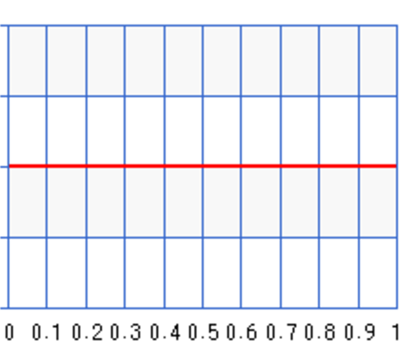
An uniform distribution maximizes the entropy (randomness) to reflect the highest uncertainty of our belief.
We use Beta function to model our belief. We set \(a=b=1\) in the beta distribution for an uniform probability distribution. The following plots the distribution \(P(\theta)\):
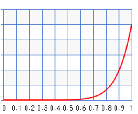
Different values of \(a\) and \(b\) result in different probability distribution. For \(a=10, b=1\), the probability peaks towards \(\theta=1\) :
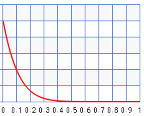
For \(a=1, b=10\), the probability peaks towards \(\theta=0\):
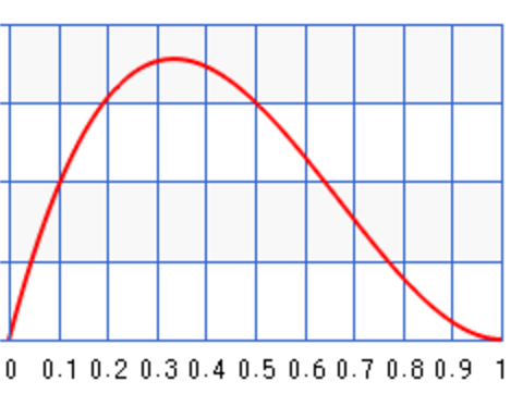
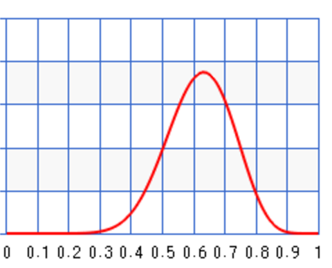
For example, we can start with some prior information about the infection rate of the flu. For example, for \(a=2, b=3\), we set the peak around 0.35:
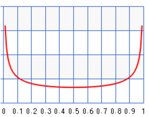
For \(a=b=0.5\):
We model the likeliness \(P(data \vert \theta)\) of our observed data given a specific infection rate with a Binomial distribution. For example, what is the possibility of seeing 4 infections (variable x) out of 10 (N) samples given the infection rate \(\theta\).
\[\begin{align} P(data \vert \theta) & = {N \choose x} \theta^{x} (1-\theta)^{N-x} \end{align}\]Let’s apply the Bayes theorem to calculate the posterior \(P(\theta \vert data)\): the probability distribution function for \(\theta\) given the observed data. We usually remove constant terms from the equations because we can always re-normalize the graph later if needed.
\[\begin{align} P(data \vert \theta) & \propto \theta^x(1-\theta)^{N-x} & \text{ (model with a Binomial distribution) }\\ P(\theta) & \propto \theta^{a-1} (1-\theta)^{b-1} & \text{ (model as a beta distribution) }\\ \end{align}\]Using Bayes’ theorem:
\[\begin{align} P(\theta \vert data) & = \frac{P(data \vert \theta) P(\theta)}{P(data)} \\ & \propto P(data \vert \theta) P(\theta) \\ & \propto \theta^{a + x -1} (1-\theta)^{N + b -x -1} \\ & = B(a+x, N + b - x) \end{align}\]We start with a Beta function for the prior and end with another Beta function as the posterior. Pior is a conjugate prior if the posterior is the same class of function as the prior. As shown below, this helps us to calculate the posterior much easier.
We start with the uniformed distributed prior \(P(\theta) = B(1, 1)\) assuming we have no prior knowledge on the infection rate. \(\theta\) is equally likely for any values between [0, 1].
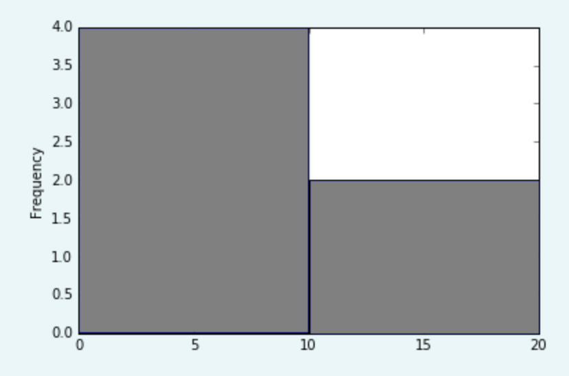
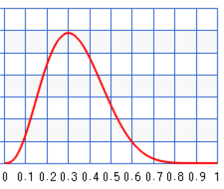
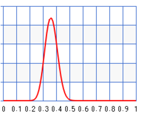
For the first set of sample, we have 3 infections our of a sample of 10. (\(N=10, x=3\)) The posterior will be \(B(1+3, 10 + 1 - 3) = B(4, 8)\) which has a peak at 0.3. Even assuming no prior knowledge (an uniform distribution), Bayes’ theorem arrives with a posterior peaks at the maximum likeliness estimation (0.3) from the first sample data.
Just for discussion, we can start with a biased prior \(B(10, 1)\) which peak at 100% infection:
The observed sample (\(N=10, x=3\)) will produce the posterior:
\(B(a+x, N + b - x) = B(10+3, 10 + 1 - 3) = B(13, 8)\) with \(\theta\) peak at 0.62.
Let’s say a second set of samples came in 1 week later with \(N=100, x=30\). We can update the posterior again.
\[B(10+30, 100 + 1 - 30) = B(40, 71)\]As shown, the posterior’s peak moves closer to the maximum likeliness to correct the previous bias.
When we enter a new flu season, our new sampling size for the new Flu strain is small. The sampling error can be large if we just use this small sampling data to compute the infection rate. Instead, we use prior knowledge (the last 12 months data) to compute a prior for the infection rate. Then we use Bayes theorem with the prior and the likeliness to compute the posterior probability. When data size is small, the posterior rely more on the prior but once the sampling size increases, it re-adjusts itself to the new sample data. Hence, Bayes theorem can give better prediction.
Given datapoints \(x^{(1)} , \dots , x^{(m)}\), we can compute the probability of \(x^{(m+1)}\) by integrating the probability of each \(\theta\) with the probability of \(x^{(m+1)}\) given for each \(\theta\). i.e. the expected value \(\mathbb{E}_θ [ p(x^{(m+1)} \vert θ) ]\).
\[p(x^{(m+1)} \vert x^{(1)} , \dots , x^{(m)}) = \int p(x^{(m+1)} \vert θ) p( θ \vert x^{(1)} , \dots , x^{(m)}) dθ \\\]Dirac distribution
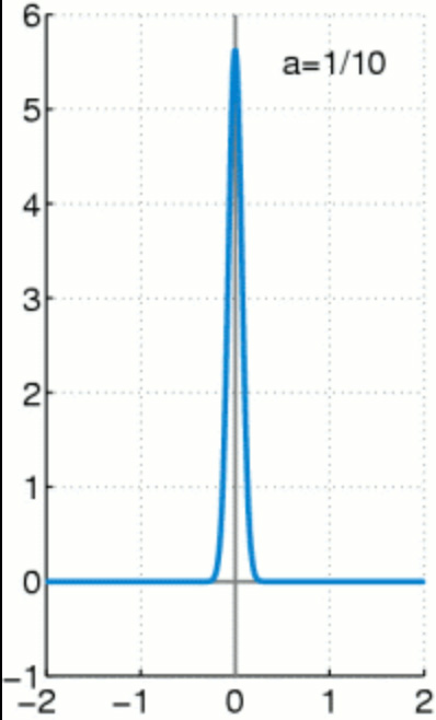
Dirac distribution models a distribution with value sharply located at \(\mu\).
Exponential and Laplace distribution
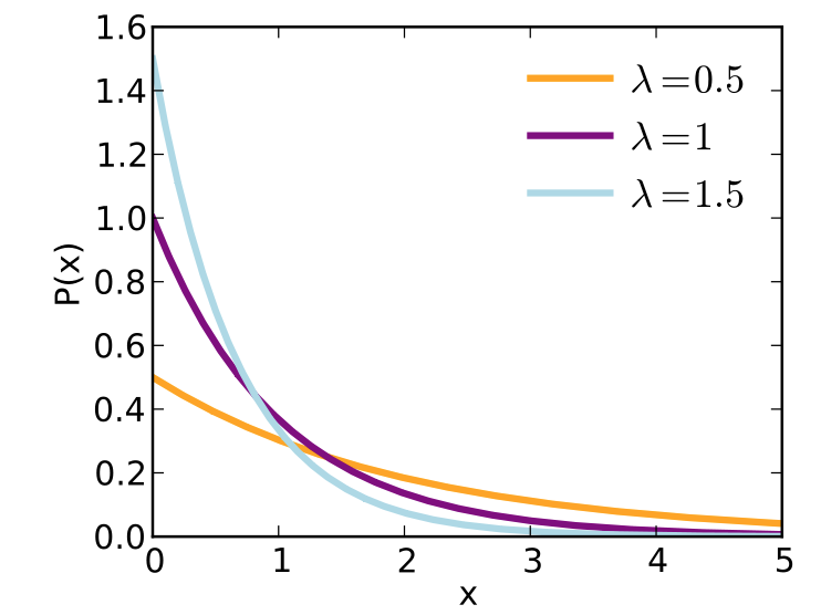
Both exponential and Laplace distribution have a sharp point at 0 which is sometimes used for machine learning.
Exponential distribution:
(Source Wikipedia)
\[p(x;\lambda)= \begin{cases} \lambda e^{- \lambda x} & x ≥ 0 \\ 0 & x < 0 \\ \end{cases}\]Laplace distribution:
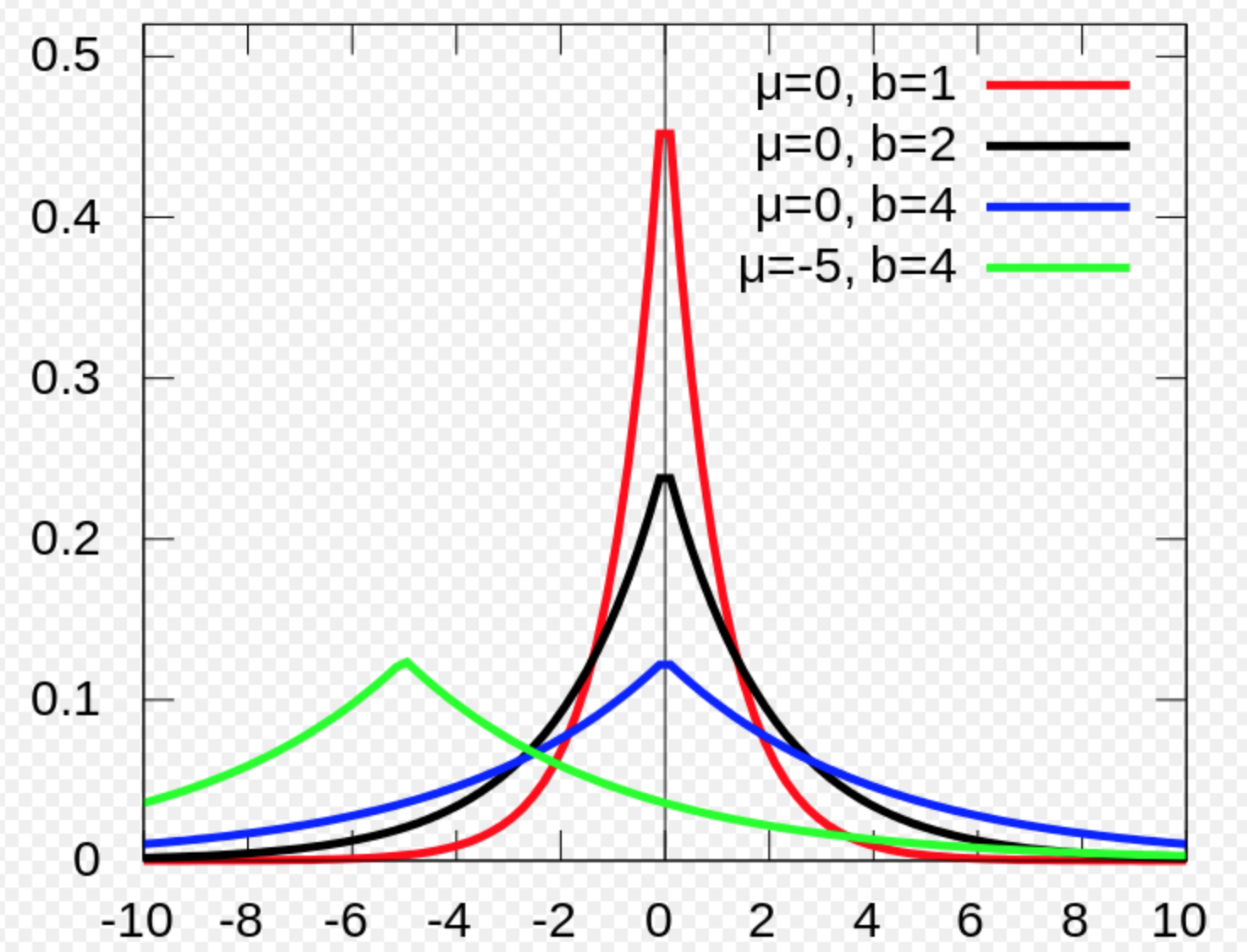
Examples
Calculate bias and variances of a Gaussian distribution estimator
Gaussian equation:
\[\mathcal{N}(x;μ, σ^2) = \frac{1}{\sigma\sqrt{2\pi}}e^{-(x - \mu)^{2}/2\sigma^{2} }\]A common estimator for the Gaussian mean parameter by sampling \(m\) datapoints:
\[\begin{split} \hat{\mu}_m = \frac{1}{m} \sum^m_1 x^{(i)} \\ \end{split}\]Estimate the Bias of the estimator:
\[\begin{split} bias(\hat{\mu}_m ) &= \mathbb{E}[\hat{\mu}_m ] - \mu \\ &= \mathbb{E} [\frac{1}{m} \sum^m_1 x^{(i)} ] - \mu \\ &= \frac{1}{m} \mathbb{E} [\sum^m_1 x^{(i)} ] - \mu \\ &= \frac{1}{m} m \mathbb{E}[x^{(i)}] - \mu \\ &= \mu - \mu \\ &= 0 \\ \end{split}\]Hence, our estimator for the Gaussian mean parameter has zero bias.
Let’s consider the following estimator for the Gaussian variance parameter:
\[\begin{split} \hat{\sigma}^2_m = \frac{1}{m} \sum^m_{i=1} (x^{(i)} - \hat{\mu_m})^2 \\ \end{split}\]Estimate the Bias of the estimator:
\[\begin{split} bias(\hat{\sigma}^2_m) = \mathbb{E} [\hat{\sigma}^2_m] - \sigma^2 \end{split}\]Calculate \(\mathbb{E} [\hat{\sigma}^2_m]\) first:
\[\begin{split} \mathbb{E} [\hat{\sigma}^2_m] & = \mathbb{E} [\frac{1}{m}\sum_{i = 1}^m (x^{(i)} - \mu_m)^2] = \frac{1}{m} \mathbb{E} [\sum_{i = 1}^m ((x^{(i)})^2 - 2x^{(i)} \mu_m + \mu_m^2)] \\ & = \frac{1}{m} \big( \mathbb{E} [\sum_{i = 1}^m (x^{(i)})^2] - \mathbb{E} [\sum_{i = 1}^m 2x^{(i)} \mu_m] + \mathbb{E} [\sum_{i = 1}^m \mu_m^2)] \big) \\ & = \frac{1}{m} \big( \mathbb{E} [\sum_{i = 1}^m (x^{(i)})^2] - \mathbb{E} [\sum_{i = 1}^m 2 \mu_m \mu_m] + \mathbb{E} [\sum_{i = 1}^m \mu_m^2)] \big) \\ &= \frac{1}{m} \big( \mathbb{E} [\sum_{i = 1}^m (x^{(i)})^2] - \mathbb{E} [\sum_{i = 1}^m \mu_m^2)] \big) \\ &= \mathbb{E} [x_m^2] - \mathbb{E} [\mu_m^2)] \\ & = \sigma_{x_m}^2 + \mu_{x_m}^2 - \sigma_{\mu_m}^2 - \mu_{\mu_m}^2 \quad \text{since }\sigma^2 = \mathbb{E} [x^2] - \mu^2 \implies \mathbb{E} [x^2] = \sigma^2 + \mu^2 \\ & = \sigma_{x_m}^2 - \sigma_{\mu_m}^2 \quad \text{since } \mu_{x_m}^2 = \mu_{\mu_m}^2 \\ & = \sigma_{x_m}^2 - Var(\mu_m) \\ & = \sigma_{x_m}^2 - Var( \frac{1}{m} \sum^m_{i=1} x^m) \\ & = \sigma_{x_m}^2 - \frac{1}{m^2} Var(\sum^m_{i=1} x^m) \\ & = \sigma_{x_m}^2 - \frac{1}{m^2} m \sigma_{x^m}^2 \\ & = \frac{m-1}{m} \sigma_{x^m}^2 \neq \sigma^2_{x^m}\\ \end{split}\]Hence, this estimator is biased. Intuitively, we sometimes over-estimate and sometimes estimate \(\mu\). By squaring it, we tends to over-estimate all the time and therefore the estimator has biases. The correct estimator for \(\sigma\) is:
\[\begin{split} \hat{\sigma}^2_m = \frac{1}{m-1} \sum^m_{i=1} (x^{(i)} - \mu_m)^2 \\ \end{split}\]Proof:
\[\begin{split} \mathbb{E} [\hat{\sigma}^2_m] & = \mathbb{E} [ \frac{1}{m-1} \sum^m_{i=1} (x^{(i)} - \mu_m)^2 ] \\ & = \frac{1}{m-1} \mathbb{E} [ \sum^m_{i=1} (x^{(i)} - \mu_m)^2 ] \\ & = \frac{1}{m-1} (m-1) \mathbb{E} [ \sigma^2_{x_m}] \quad \text{reuse the result from the calculations of } \mathbb{E} [\hat{\sigma}^2_m]. \\ & = \sigma^2_{x_m} \\ \end{split}\]Calculate bias and variances of a Bernoulli Distribution estimator
Bernoulli Distribution:
\[P(x^{(i)}; θ) = θ^{x^{(i)}} (1 − θ)^{(1−x^{(i)} )}.\]A common estimator will be:
\[\hat{θ}_m = \frac{1}{m} \sum^m_{i=1} x^{(i)}\]Find the bias:
\[\begin{split} bias(\hat{θ}_m) &= \mathbb{E} [\hat{θ}_m] - θ \\ &= \mathbb{E} [ \frac{1}{m} \sum^m_{i=1} x^{(i)} ] - θ \\ &= \frac{1}{m} (\sum^m_{i=1} \mathbb{E} [ x^{(i)} ]) - θ \\ &= \frac{1}{m} (\sum^m_{i=1} (\sum^1_0 θ^{x^{(i)}} (1 − θ)^{(1−x^{(i)} )})) - θ \\ &= \frac{1}{m} (\sum^m_{i=1} θ) - θ \\ &= \frac{1}{m} m θ - θ \\ &= 0 \end{split}\]i.e. our estimator has no bias.
The variance of \(θ\) drops as \(m\) increases:
\[\begin{split} Var(\hat{θ}_m) &=Var( \frac{1}{m} \sum^m_{i=1} x^{(i)} ] ) \\ &= \frac{1}{m^2} \sum^m_{i=1} Var (x^{(i)} ]) \\ &= \frac{1}{m^2} \sum^m_{i=1} θ(1-θ)\\ &= \frac{1}{m^2} m θ(1-θ)\\ &= \frac{1}{m} θ(1-θ)\\ \end{split}\]