“Machine learning - Restricted Boltzmann Machines.”
Maxwell–Boltzmann distribution
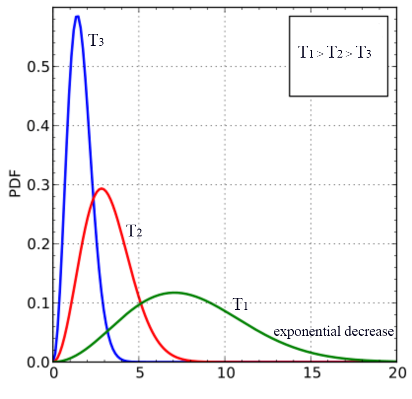
Maxwell–Boltzmann distribution models the distribution of speeds of the gas molecules at a certain temperature:
(Source Wikipedia)
Here is the Maxwell–Boltzmann distribution equation:
\[\begin{split} f(v) & = \sqrt{ \left (\frac{m}{2\pi kT} \right)^{3} } 4\pi v^2 e^{\frac{-mv^2}{2kT}} \\ \end{split}\]\(f(v)\) gives the probability density function (PDF) of molecules with velocity \(v\) which is a function of the temperature \(T\). The probability density decreases exponentially with \(v\). As the temperature increases, the probability of a molecule with higher velocity also increases. But since the number of molecules remains constant, the peak is therefore lower.
Energy based model
In Maxwell–Boltzmann statistics, the probability distribution is defined using an energy function \(E(x)\):
\[\begin{split} P(x) & = \frac{e^{-E(x)}}{Z} \\ \end{split}\]where
\[Z = {\sum_{x^{'}} e^{-E(x^{'}) }}\]Z is sum from all possible states and it is called the partition function. It renormalizes the probability between 0 and 1.
By defining an energy function \(E(x)\) for an energy based model like the Boltzmann Machie or the Restricted Boltzmann Machie, we can compute its probability distribution \(P(x)\).
Boltzmann Machine
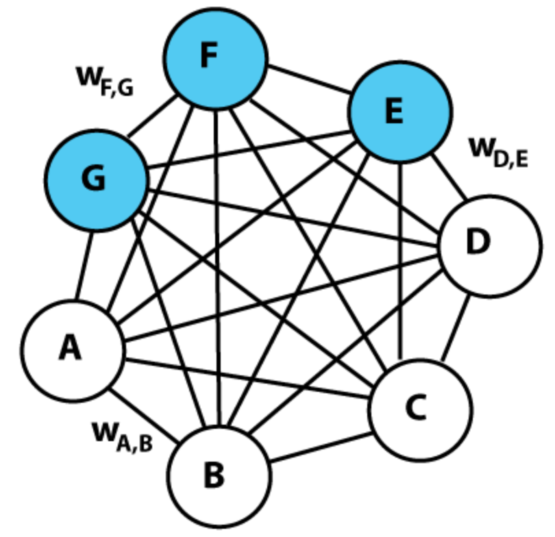
A Boltzmann Machine projects an input data \(x\) from a higher dimensional space to a lower dimensional space, forming a condensed representation of the data: latent factors. It contains visible units (\(A, B, C, D, \dots\)) for data input \(x\) and hidden units (blue nodes) which are the latent factors of the input \(x\). All nodes are connected together with a bi-directional weight \(W_{ij}\).
(Source Wikipedia)
Each unit \(i\) is in a binary state \(s_i \in \{0, 1 \}\). We use \(W_{ij}\) to model the connection between unit \(i\) and \(j\). If \(s_i\) and \(s_j\) are the same, we want \(W_{ij}>0\). Otherwise, we want \(W_{ij}<0\). Intuitively, \(W_{ij}\) indicates whether two units are positively or negatively related. If it is negatively related, one activation may turn off the other.
The energy between unit \(i\) and \(j\) is defined as:
\[E(i, j) = - W_{ij} s_i s_j - b_i s_i\]Hence as indicated, the energy is increased if \(s_i = s_j = 1\) and \(W_{ij}\) is wrong (\(W_{ij} <0)\). The likelihood for \(W_{ij}\) decreases as energy increases.
The energy function of the system is the sum of all units:
\[\begin{split} E &= - \sum_{i < j} W_{ij}s_i s_j - \sum_i b_i s_i \quad \text{ or} \quad E(x) & = -x^T U x - b^T x \\ \end{split}\]The energy function is equivalent to the cost function in deep learning.
Using Boltzmann statistics, the PDF for \(x\) is
\[\begin{split} P(x) & = \sum_{x^{'}} P(x, x^{'}) \\ & = \sum_{x^{'}} \frac{e^{-E(x, x^{'})}}{Z} \\ \end{split}\]where \(x^{'}\) are all the neighboring units.
Restricted Boltzmann Machine (RBM)
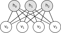
In Boltzmann Machines, visible units or hidden units are fully connected with each other. In Restricted Boltzmann Machine (RBM), units in the same layer are not connected. The units in one layer is only fully connected with units in the next layer.
(Source)
The energy function for an RBM:
\[E(v, h) = - \sum_{i \in visible} a_i v_i - \sum_{j \in hidden} b_j h_j - \sum_{i, j} v_i h_j W_{ij} \\\]In vector form:
\[\begin{split} E(v, h) = -a^T v - b^T h - v^T W h \\ \end{split}\]Probability for a pair of visible and hidden unit:
\[\begin{split} P(v, h) & = \frac{1}{Z} e^{-E(v, h)} \\ \end{split}\]where the partition function \(Z\) is:
\[Z = {\sum_{v, h} e^{-E(v, h) }}\]Probability for a visible unit (summing over all neighbors):
\[\begin{split} P(v) &= \frac{1}{Z} \sum_h e^{-E(v, h)} \end{split}\]The probability that the model is assigned to a training image can be raised by lower the energy of that image and to raise the energy of other images. The derivative of the log probability of a training vector can be find to be:
\[\frac{\partial \log p(v)}{\partial w_{ij} } = \langle v_i h_j \rangle_{data} - \langle v_i h_j \rangle_{model}\]which \(\langle v_i h_j \rangle_{data}\) is the expectation value for \(v_i h_j\) with \(v\) from the training samples. However, the \(v\) in \(\langle v_i h_j \rangle_{model}\) is sample from the model i.e. \(v \sim P_{model}(v) = \frac{1}{Z} \sum_h e^{-E(v, h)}\). Hence, the network has the highest probability if the expected value for \(v_i h_j\) of the model matches with that of the training samples.
And during training, we can adjust the weight by:
\[\Delta w_{ij} = \epsilon (\langle v_i h_j \rangle_{data} - \langle v_i h_j \rangle_{model})\]To calculate \(\langle v_i h_j \rangle_{data}\), we sample an image from the training dataset, the binary state \(h_j, v_j\) is set to 1 with probability:
\[\begin{split} P(h_j = 1 \vert v) &= \sigma \big( b_j + \sum_i W_{ij} v_i \big) \\ P(v_i = 1 \vert h) &= \sigma \big( a_i + \sum_j W_{ij} h_j \big) \\ \end{split}\]To calculate \(\langle v_i h_j \rangle_{model}\) is hard because \(Z\) is unknown.
One possibility is to use Gibbs sampling (which will not be covered here). The other is to use approximation and \(\Delta w_{ij}\) becomes:
\[\Delta w_{ij} = \epsilon (\langle v_i h_j \rangle_{data} - \langle v_i h_j \rangle_{reconstruct})\]First we pick \(v\) from the training samples. Then the probability of the hidden units are computed and we sample a binary value from it. Once the binary states \(h_j\) have been chosen for the hidden units, a reconstruction \(v_i\) is produced by the \(h_j\).
To train the biases, the steps are similar except we use the individual state \(v_i\) or \(h_j\) instead.
Simple walk through
- Start with a sample \(v\) from the training dataset.
- Compute \(p(h \vert v) = \sigma(b_j + \sum_i v_i w_{ij})\) and sample \(h \in \{ 0, 1\}\) from it.
- \(positve_{ij} = v_i h_j\).
- Compute \(p(v^{(1)} \vert h) = \sigma(a_i + \sum_j h_j w_{ij})\) and sample \(v^{(1)}\in \{ 0, 1\}\) from it.
- \(negative_{ij} = v^{(1)}_i h_j\).
- \(W_{ij} = W_{ij} + \epsilon (positive_{ij} - negative_{ij})\).
Free energy
The free energy of visible vector \(v\) is the energy of a single configuration that has the same probability as all of the configurations that contain \(v\):
\[e^{-F(v)} = \sum_h e^{-E(v, h)}\]which is also the expected energy minus the entropy:
\[F(v) = - \sum_{i \in visible} v_i a_i - \sum_{j \in hidden} p_j x_j + \sum_j \big( p_j \log p_j + (1-p_j) \log(1-p_j) \big)\]where \(x_j\) is the total input to hidden unit \(j\).
\[x_j = b_j + \sum_i v_i w_{ij} \\ p_j = \sigma(x_j)\]The free energy of RBM can be simplified as:
\[\begin{split} F(v) & = - log \sum_{h \in \{0, 1\}^m} e^{-E(v, h)} \\ & = - log \sum_{h \in \{0, 1\}^m} e^{ h^T W v + a^T v + b^T h} \\ & = - log \big( e^{a^Tv} \sum_{h \in \{0, 1\}^m} e^{ h^T W v + b^T h} \big) \\ & = - a^Tv - log \Big( \big( \sum_{h_1 \in \{ 0, 1 \} } e^{ h_1 W_1 v + b_1h_1} \big) + \dots + \big( \sum_{h_m \in \{ 0, 1 \}} e^{ h_m W_m v + b_mh_m} \big) \Big)\\ & = - a^Tv - log \Big( \big( e^{ 0 W_1 v + b_1 0} + e^{ 1 W_1 v + b_1 1} \big) + \dots + \big( e^{ 0 W_m v + b_m 0} + e^{ 1 W_m v + b_m 1} \big) \Big)\\ & = - a^Tv - log \Big( \big( 1 + e^{W_1 v + b_1} \big) + \dots + \big( 1 + e^{W_m v + b_m} \big) \Big)\\ & = - a^Tv - \sum_j \log(1 + e^{W_j v + b_j}) \\ & = - a^Tv - \sum_j \log(1 + e^{x_j}) \\ \end{split}\]Energy based model (Gradient)
Recall:
\[\begin{split} P(x) & = \sum_{x^{'}} \frac{e^{-E(x, x^{'})}}{Z} \\ e^{-\mathcal{F}(x) } & = \sum_{x^{'}} e^{-E(x, x^{'})} \\ \end{split}\]Therefore:
\[\begin{split} P(x) &= \frac{e^{-\mathcal{F}(x)}}{Z} \quad \text{where } Z = \sum_{x^{'}} e^{-\mathcal{F}(x^{'})} \\ \end{split}\]Take the negative log:
\[\begin{split} - \log P(x) & = \mathcal{F}(x) + \log Z \\ & = \mathcal{F}(x) + \log (\sum_{x^{'}} e^{-\mathcal{F}(x^{'})}) \\ \end{split}\]Its gradient is:
\[\begin{split} - \frac{\partial \log P(x)}{\partial \theta} & = \frac{\partial \mathcal{F}(x)}{\partial \theta} + \frac{1}{\sum_{x^{'}} e^{-\mathcal{F}(x^{'})}} \frac{\partial }{\partial \theta} \sum_{x^{'}} e^{-\mathcal{F}(x^{'})} \\ & = \frac{\partial \mathcal{F}(x)}{\partial \theta} - \sum_{x^{'}} \frac{e^{-\mathcal{F}(x^{'})}}{\sum_{x^{'}} e^{-\mathcal{F}(x^{'})}} \frac{\partial \mathcal{F}(x^{'})}{\partial \theta} \\ & = \frac{\partial \mathcal{F}(x)}{\partial \theta} - \sum_{x^{'}} \frac{e^{-\mathcal{F}(x^{'})}}{Z} \frac{\partial \mathcal{F}(x^{'})}{\partial \theta} \\ & = \frac{\partial \mathcal{F}(x)}{\partial \theta} - \sum_{x^{'}} p(x^{'}) \frac{\partial \mathcal{F}(x^{'})}{\partial \theta} \\ & = \frac{\partial \mathcal{F}(x)}{\partial \theta} - \mathbb{E}_{x^{'} \sim p} [ \frac{\partial \mathcal{F}(x^{'})}{\partial \theta} ] \\ \end{split}\]where \(p\) is the probability distribution formed by the model.
Contrastive Divergence (CD-k)
For a RBM,
\[F(v) = - \sum_i v_i a_i - \sum_j \log(1 + e^{x_j})\]where
\[x_j = b_j + \sum_i v_i w_{ij} \\\]i.e.
\[F(v) = -a v - \sum_{i \in visible} \log(1 + e^{b_i + W_i v})\](Without proof) We combine \(F(v)\) with the gradient from the last section, :
\[\begin{split} - \frac{\partial \log P(x)}{\partial W_{ij}} & = \mathbb{E} [ p(h_j \vert v) v_i ] - v^{(k)}_i \sigma(W_j v^{(k)} + b_j ) \\ - \frac{\partial \log P(x)}{\partial b_j} & = \mathbb{E} [ p(h_j \vert v) ] - \sigma(W_j v^{(k)} ) \\ - \frac{\partial \log P(x)}{\partial a_i} & = \mathbb{E} [ p(v_i \vert h) ] - v^{(k)}_i \\ \end{split}\]which
\[h ^{(k)} \sim \sigma(W v^{(k)} + b) \\ v ^{(k+1)} \sim \sigma(W h^{(k)} + a) \\\]\(v = v^{(0)}\) and \(h^{(1)}\) is the prediction from \(v^{(0)}\), \(v^{(1)}\) is the prediction from \(h^{(1)}\).
So we sample an image from the training data as \(v\) and compute \(v^{(k)}\). In practice, \(k=1\) will show resonable result already.
Credit
For those interested in the technical details in the Restricted Boltzmann Machines, please read A Practical Guide to Training Restricted Boltzmann Machines from Hinton.