“Machine learning - Decision tree, Random forest, Ensemble methods and Beam searach”
Decision Tree
A decision tree is a binary tree:
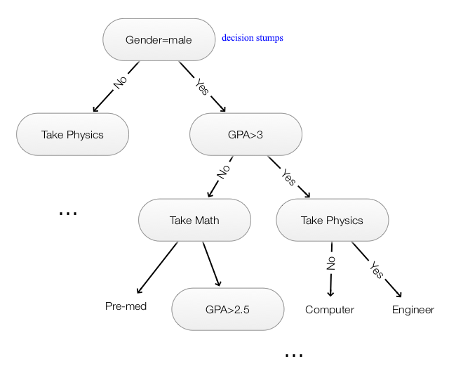
- Each node partitions data according to a splitting rule. (For example, GPA>3)
- Leaf node returns a label for the classification. (Engineer)
Decision stumps:
- Splitting rule based on thresholding one feature (GPA>3)
- Select the rule with the highest accuracy in predicting a label, or
- Select the rule that reduce the entropy the most
- Greedy recursive splitting makes 1 stump at a time
- Can re-use features to split a tree (GPA>2.5)
- Risk overfitting as the depth of the tree increases
Splitting based on entropy
Entropy measure randomness. High entropy means more randomness.
\[H(y) = - \sum_X p(y) \log p(y)\]In decision tree, we want a split that make data most predictable. Therefore, we are going to pick a rule that have the highest drop in entropy.
\[H(Engineer) - H(Engineer \vert GPA>3) \\\] \[H(Engineer) - H(Engineer \vert GPA>2.5) \\\]Gini
Let’s say a class have 30 students. 15 students (50%) go to an Engineering school. The class has 10 female students and 4 go to the Engineering school (40%). The class has 20 male students and 11 goes to the engineer school.
Let’s calculate the Gini value based on splitting by gender: Gini value is calculated as
\[1 - p^2 - (1-p)^2\]For the sub-node Female, 40% goes to the engineer school. So \(Gini_f = 1 - 0.4 * 0.4 + 0.6 * 0.6\).
For the sub-node Male, 55% goes to the engineer school. So \(Gini_m = 1- 0.55 * 0.55 + 0.45 * 0.45\).
Weighted \(Gini = (\frac{10}{30} Gini_f + \frac{20}{30} Gini_m )\) (10 out of 30 students are female.)
We can make another calculation with another splitting rule like (GPA>3.0). The one with the highest weighted Gini should be used for the splitting.
Chi-square
Split on Gender:
| Node | Engr. | Not engr. | Total | Expected* | Not Expected* | Engr. deviation | Non-engr deviation |
| Female | 4 | 6 | 10 | 5 | 5 | -1 | 1 |
| Male | 11 | 9 | 20 | 10 | 10 | 1 | -1 |
* We calculate the expected value from the parent’s probability distribution. From the parent node, 50% are engineerings. So the expected value for female engineer is \(10 * 0.5 = 5\).
Chi-square for Female as engineers:
\[\text{chi-square}_{\text{female as engr}} = \frac{(actual – expected)^2} {expected^{1/2}}\]Chi-square for Female not as engineers:
\[\text{chi-square}_{\text{female not as engr}} = \frac{(\text{not actual engr} – \text{not expected})^2} {\text{not expected}^{1/2}}\]The total chi-square is :
\[\text{chi-square}_{\text{female as engr}} + \text{chi-square}_{\text{female not as engr}} + \text{chi-square}_{\text{male as engr}} + \text{chi-square}_{\text{male not as engr}}\]The final split rule is to pick one with the highest total chi-square.
Ensemble methods
We start with a shallow decision tree and gradually increase its depth to improve the model accuracy. However, at some point, we start overfitting the model and hurting the generalization. Finding a balance between overfitting and model complexity can be hard. Alternatively, we can adopt a simpler model and push the accuracy by not taking decision from just one model but many models. Even each model makes some mistakes, the chance that all make the same mistakes is small. Hence we ensemble simpler models to avoid overfitting and later combining all results to make a much accurate prediction.
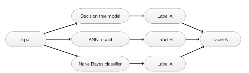
Averaging
- Make predictions by multiple models
- Models built with different initial parameters or
- Collect models at different iterations of the same training or
- Models from different methods (KNN, decision trees, naive bayes … )
- Use simple majority vote, averaging probability (for scholastic model) or weighted average
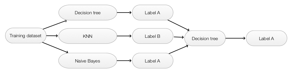
Stacking
- Models can be built with different methods (KNN, decision trees, naive bayes … )
- The predictions of each model are used as the input feature of another model
Boosting
To avoid overfitting, we ensemble many simpler models to make predictions. We start with a training dataset to build the first model. For the next model, we sample the training datasets giving more weight on those mislabeled datapoints. This force the next iteration to address what we miss in our first model. After many iterations, we build many different rules that when combined becomes very powerful.
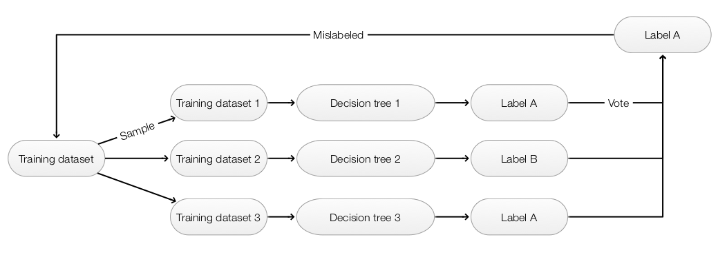
- Use a simple model that it is hard to overfit (For example, a shallow decision tree)
- Fit the model with the training data
- For datapoints that are mis-labeled by \(Model_i\), we assign a higher weight to them.
- Sample the next training datapoints based on the assigned weight
- Fit a new model with the new training dataset
- Continue the process when enough models are built
- Make prediction using ensemble methods
Random forest
Random forest is an ensemble methods by building many decision trees using bootstrap sample and random tree.
Bootstrap sample
- Build many training datasets with sampling from the original training dataset with replacement
- Since this is sampling with replacement, the new dataset will have duplicate and missing datapoints
- About 63% of original data will be included in each new dataset
- Fit multiple models using different datasets above
- Averaging the prediction
Random tree
- In selecting a splitting rule at each node, we do not try out all possible features
- Instead, we randomly select a sub-set of features for consideration
- Different nodes may have a different sub-set of features to determine the splitting rule
- By dropping features, we can build a deeper tree before overfitting hurts us
- Averaging the predictions to increase accuracy
Local beam search
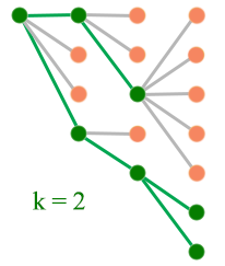
- Start from an initial state
- Explore all the successors of all the states
- If any of the state is the goal state, stop
- Otherwise, select the best k successors (green dots) and explore all successors
- Re-iterate again by picking best k successors