“Machine learning - Hidden Markov Model (HMM)”
Hidden Markov Model (HMM)
There are hidden states of a system that we cannot observe directly. 20% chance that we go to watch a movie when we are happy but also 40% chance when we are upset. People may tell you what they did (observable) but unlikely tell you the truth whether they were happy or upset (the hidden state). Given the information on the chance of what people do when they are upset or happy, we can uncover the hidden state (happy or upset) by knowing what they did.
Prior belief: Here is our belief on the chance of being happy and upset.
\[\begin{split} x & \in {happy, upset} \\ P(happy) &= 0.8 \\ P(upset) &= 0.2 \\ \end{split}\]Observables (what we do):
\[y \in {movie, book, party, dinning}\]Here is the likelihood: the chance of what will we do when we are happy or upset.
| movie | book | party | dinning | |
| Given being happy | 0.2 | 0.2 | 0.4 | 0.2 |
| Given being upset | 0.4 | 0.3 | 0.1 | 0.2 |
Compute the posterior:
\[\begin{split} P(x \vert y) &= \frac{P(y \vert x) P(x)}{P(y)} \\ P(happy \vert party) &= \frac{P(party \vert happy ) P(happy)} {P(party)} \\ P(happy \vert party) &= \frac{P(party \vert happy ) P(happy)} {P(party \vert happy) P(happy) + P(party \vert upset) P(upset)} \\ & = \frac{0.4 * 0.8}{0.4*0.8 + 0.1* 0.2} = 0.94 \end{split}\]Hence, the chance that a person goes to party because he/she is happy is 94%. This is pretty high because we have a high chance of being happy and also high chance to go party when we are happy.
In reality, being happy or upset is not independent. Instead, it can be better model by a Markov Model. Here is the transition probability from \(x_t\) to \(x_{t+1}\).
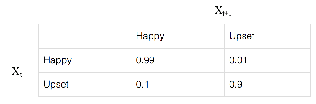
For example,
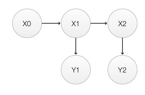
\[P(Happy_{t+1} \vert Happy_t) = 0.99\]he Markhov process for 2 timesteps is:
To recap,
\(P(x_0)\):
\[\begin{split} P(x_0=happy) & =0.8 \\ P(x_0=upset) & =0.2 \\ \end{split}\]\(P(x_{t+1} \vert x_t)\):
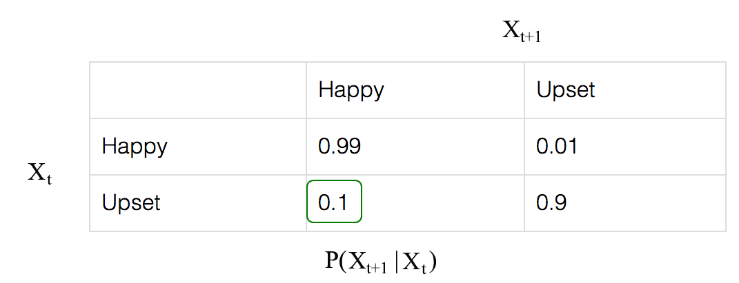
\(P( y_t \vert x_t)\):
| movie | book | party | dinning | |
| Given being happy | 0.2 | 0.2 | 0.4 | 0.2 |
| Given being upset | 0.4 | 0.3 | 0.1 | 0.2 |
Our objective is to calculate:
\[\begin{split} P(x_t \vert y_{1:t} ) &= P(x_t \vert y_1, y_2, \cdots, y_t) \\ y_1 & \rightarrow P(x_1 \vert y1) \\ y_2 & \rightarrow P(x_2 \vert y1, y2) \\ y_3 & \rightarrow P(x_3 \vert y1, y2, y3) \\ & \cdots \\ \end{split}\]Given:
\[\begin{split} P(A \vert C) & = \sum_B P(A, B \vert C) \\ P(A, B \vert C) & = P(A \vert B, C) P(B \vert C) \\ \end{split}\]We re-calculate our objective:
\[\begin{split} P(x_t \vert y_{1:{t-1}} ) & = \sum_{x_{t-1}} P(x_t, x_{t-1} \vert y_{1:{t-1}}) \\ & = \sum_{x_{t-1}} P(x_t \vert x_{t-1}, y_{1:{t-1}}) P(x_{t-1} \vert y_{1:{t-1}} ) \\ & = \sum_{x_{t-1}} P(x_t \vert x_{t-1}) P(x_{t-1} \vert y_{1:{t-1}} ) \\ \end{split}\]Given a modified Bayes’ theorem:
\[P(A \vert B, C) = \frac{P(B \vert A, C) P(A \vert C)}{ P(B \vert C)}\]To make prediction:
\[\begin{split} P(x_t \vert y_{1:t} ) & = P(x_t \vert y_{t-1}, y_{1:{t-1}} ) = P(A \vert B, C) \\ &= \frac{P(y_t \vert x_{t}, y_{1:{t-1}}) P(x_t \vert y_{1:{t-1}} )}{\sum_{x_t} P(y_t \vert x_{t}, y_{1:{t-1}}) P(x_t \vert y_{1:{t-1}} )} \\ &= \frac{P(y_t \vert x_{t} )P(x_t \vert y_{1:{t-1}} )}{\sum_{x_t} P(y_t \vert x_{t} )P(x_t \vert y_{1:{t-1}} )} \\ \end{split}\]