“Machine learning - Visualization, multi-dimensional scaling, Sammon mapping, IsoMap and t-sne”
Multi-dimensional scaling (MDS)
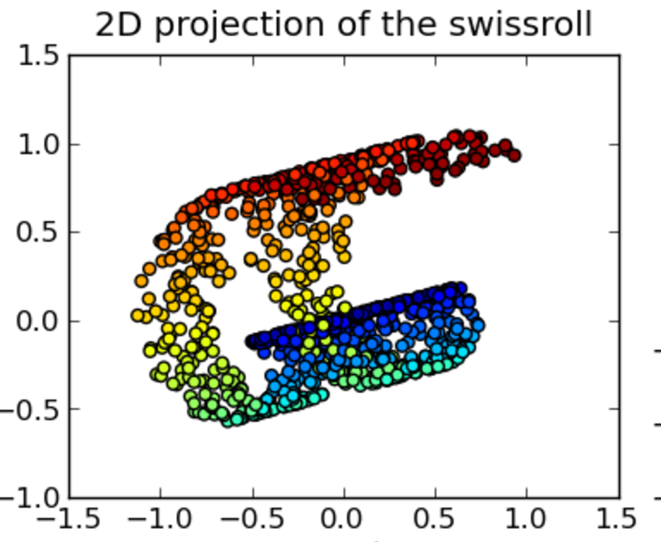
Multi-dimensional scaling helps us to visualize data in low dimension. PCA map input features from d dimensional feature space to k dimensional latent features. MDS focuses on creating a mapping that will also preserve the relative distance between data. If 2 points are close in the feature space, it should be close in the latent factor space. By enforcing such constrain, we can visualize the structure of the data in low dimension easier.
Source: wiki
Our cost function therefore penalizes the model if the relative distances are different in both spaces. In MDS, we optimize \(z\) directly with the following cost function. Usually, we use the gradient descent to solve the optimization problem.
\[\begin{split} J(z) & = \sum^n_{i=1} \sum^n_{j=i+1} (\| z_i - z_j \| - \| x_i - x_j \|)^2 \end{split}\]The cost function above measures distance by Euclidean distance. (\(dist = \| a - b \|\)) In general, the cost function can be generalized with different measurement methods:
\[J(z) = \sum^n_{i=1} \sum^n_{j=i+1} d3( d2(z_i - z_j), d1(x_i - x_j ))\]For example, we can use L1 norm which make the model less vulnerable to outliers:
\[J(z) = \sum^n_{i=1} \sum^n_{j=i+1} d3(\vert z_i - z_j \vert, \vert x_i - x_j \vert)\]Sammon mapping
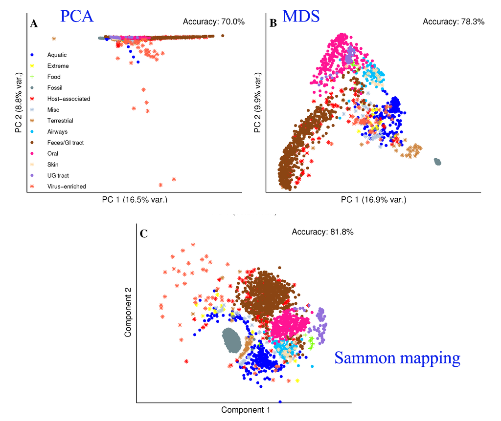
Missing one inch in measuring the waist is very different from missing one inch in measuring the distance from S.F. to L.A. In our previous cost function, we penalize the model in both cases equally. In Sammon mapping, the penalty is re-calibrated with the distance of the input feature space. Therefore, for small distances, we make sure we have a higher precision so we will not miss its fine structure.
\[J(z) = \sum^n_{i=1} \sum^n_{j=i+1} (\frac{ d2(z_i - z_j) - d1(x_i - x_j )}{d1(x_i - x_j )})^2\]PCA tends to clump datapoints of the same class together in a long but narrow band. Sammon mapping can retain the local fine structure better than a regular MDS.
Source: [http://www.mdpi.com/1422-0067/15/7/12364/htm]
IsoMap
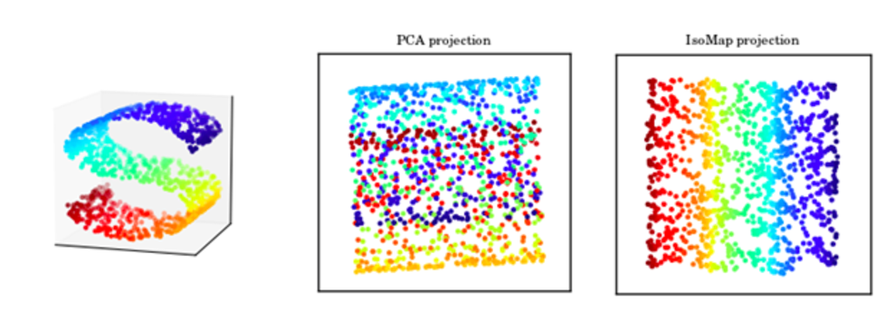
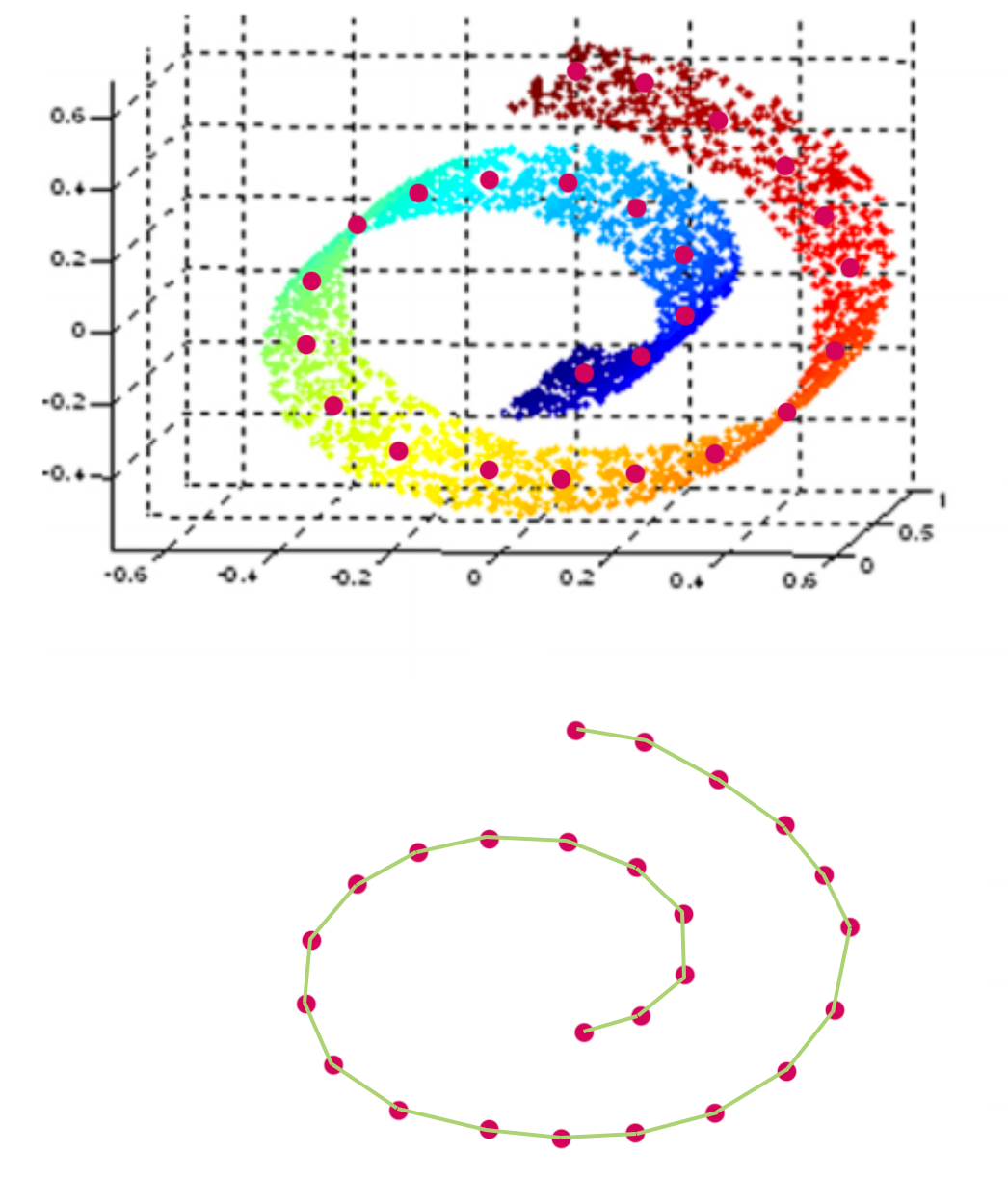
In some cases, we do not want to measure distance by Euclidean distance. For example, when we display the structure on the left below with PCA, all the color dots are meshed together even though the 3D image shows a clear spectrum of color on a S curve shape. IsoMap is a MDS method that use geodesic to measure distance so it can capture manifold structure. On the right, it is the 2D projection of the 3D S-shape manifold. In the 2D projection, we can see the color transition in the original S shape curve.
Source: [http://ciera.northwestern.edu/Education/REU/2015/Thorsen/]
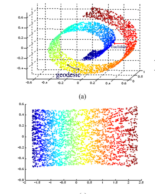
IsoMap uses geodesic rather than Euclidian space to measure distance
Source: [https://bmcbioinformatics.biomedcentral.com/track/pdf/10.1186/1471-2105-13-S7-S3?]
To visualize the “swiss-roll” manifold in 2D, we measure the geodesic distance on the manifold. We represent datapoints as nodes in a weighted graph with edges defined as the geodesic distance between 2 points.
IsoMap algorithm is:
- Find the neighbors of each point
- Points within a fixed radius
- K nearest neighbors
- Construct a graph with those nodes
- Compute neighboring edge weights (distance between neighbors)
- Compute weighted shortest path between all points
- Run MDS using the computed distance above
t-sne (t-Distributed Stochastic Neighbor Embedding)
t-sne is a MDS with special functions for d1, d2 and d3.
\[J(z) = \sum^n_{i=1} \sum^n_{j=i+1} d3( d2(z_i - z_j), d1(x_i - x_j ) )\]The distance d1 between 2 datapoints \(i, j\) in the input feature space is defined as:
\[dist_{ij} \approx \frac{\text{Similarity of i and j measured by a Gaussian distribution}}{\text{Similarity of all points measured by a Gaussian distribution}}\]The distance measured as a Gaussian distribution for point \(i\) given point \(j\) is:
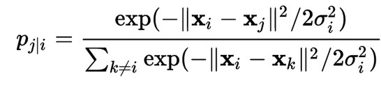
The distance between point \(i\) and \(j\).
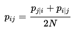
The distance d2 between 2 datapoints \(i, j\) in the latent factor space is defined as:
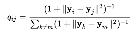
It is very similar to d1 with the exception that a Student-t distribution is used instead of the Gaussian distribution. This allows dissimilar objects to be modeled away from each other in the map.
Finally, we use the KL divergence as d3 to measure the difference between d1 and d2 distribution.
\[D_{KL}(p \vert \vert q) = \sum_{i \neq j} p_{ij} \log \frac{p_{ij}}{q_{ij}}\]Below, image features are extracted in the 4096-dimensional fc7 CNN layer and displayed in 2-D with t-sne. If we look in detail, the 2D display maintains the spatial relationship of the fc7 layer: images of the same type are cluster together. In the second picture, images with picture are cluster on the top left while dog pictures are clustered on the bottom right.
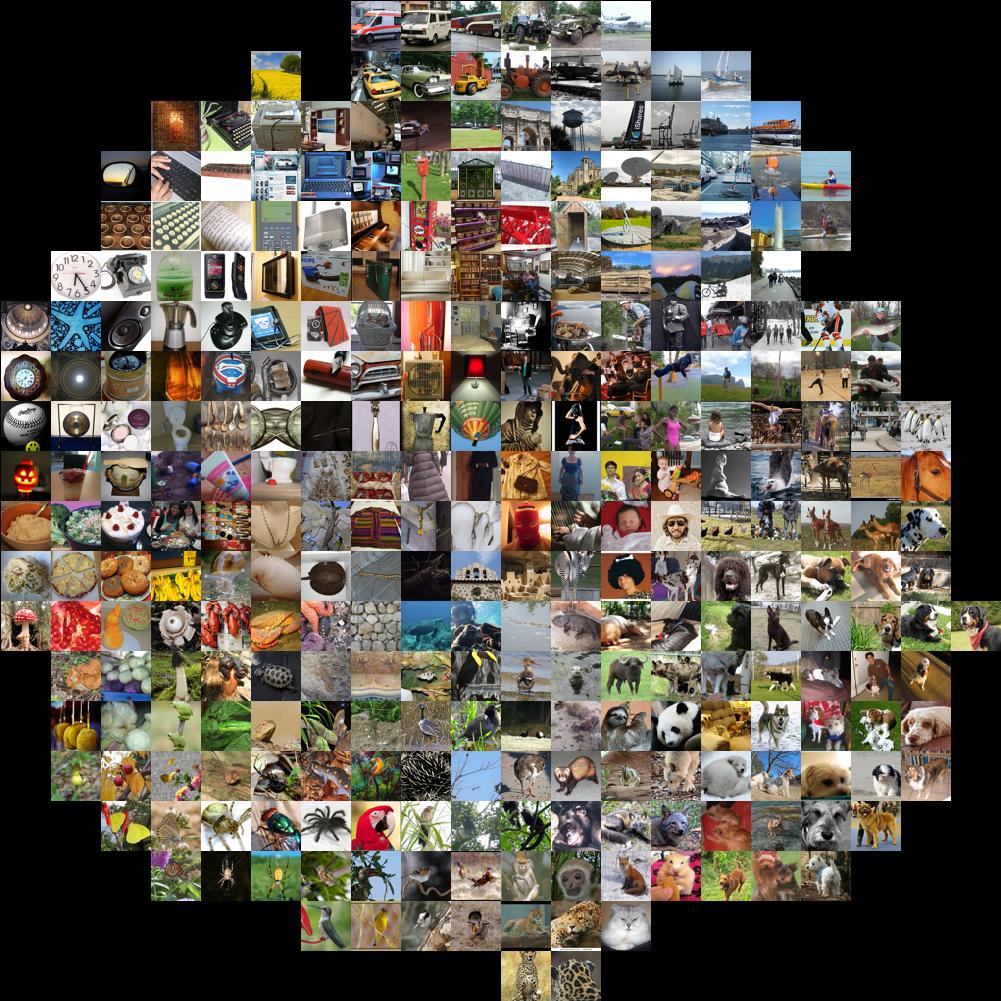
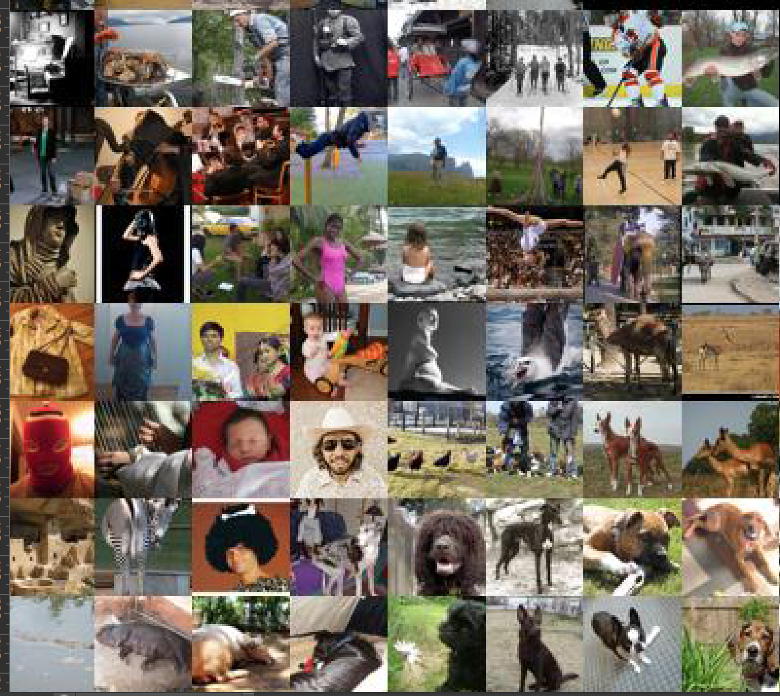
Source: [http://cs.stanford.edu/people/karpathy/cnnembed/]
Note: the challenge in MDS methods is how to space the datapoints.
- PCA tries to maximize the variance for the first principal component which the variance in the later components drop significantly. Hence, the datapoints are displayed in a long but narrow band.
- Sammon mapping use weighted cost function so large or small distances are treated with the proper precision and scale.
- ISOMAP measures distances in geodesic instead of flat plain. This allow us to explore a manifold.
- T-SNE has the advantage of Sammon mapping. Gaps are formed between different classes for better clustering.
We use Sammon mapping and T-sne method to display MNist handwriting without classified the object. The color indicates the correct class of the image. Unlike the classification method, we do not provide any labels for the training data but yet the mapping clusters them correctly as if it understands the semantic context of the image.
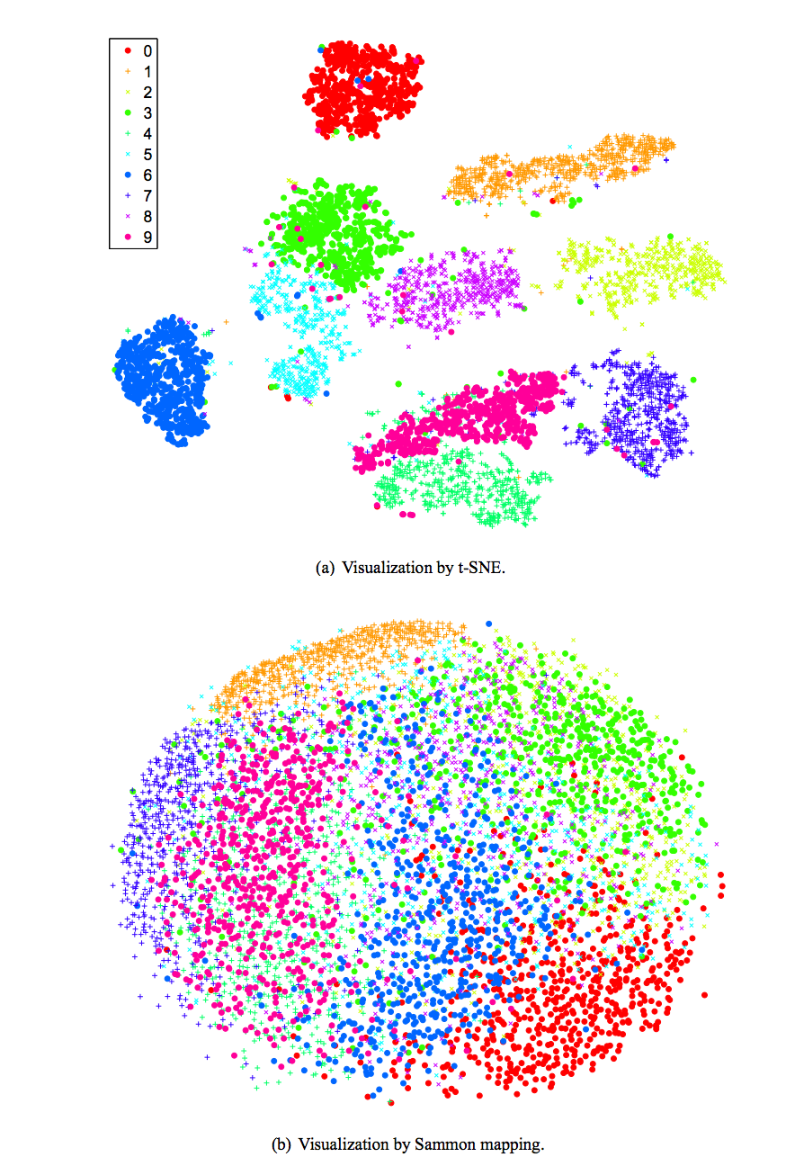
Source [http://lvdmaaten.github.io/publications/papers/JMLR_2008.pdf]