“Machine learning - PCA, SVD, Matrix factorization and Latent factor model”
Principal Component Analysis (PCA)
PCA is a linear model in mapping d-dimensional input features to k-dimensional latent factors (k principal components).
\[\begin{split} x_{ij} & = w^T_j z_i \\ \\ x_{ij} & = w_{1j} z_{i1} + w_{2j} z_{i2} + \cdots + w_{kj} z_{ik} \\ \end{split}\]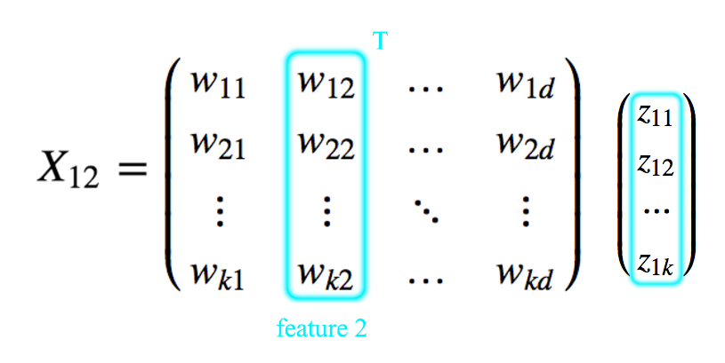
Notation:
\[\text{which } w_j \text{ is column } j \text{ of } W. \\ \text{and } w_{c_i} \text{ is row } c_i \text{ of } W. \\\]Dimension reduction can be used for data compression or visualization.
Example
For example, here is the \(W\) to match a RGB pixel to one of the 4 color palete:
\[z = \begin{pmatrix} 0 \\ 0 \\ 1 \\ 0 \\ \end{pmatrix}, \quad W = \begin{pmatrix} R_1 & G_1 & B_1\\ R_2 & G_2 & B_2\\ R_3 & G_3 & B_3\\ R_4 & G_4 & B_4\\ \end{pmatrix}\] \[\begin{split} x_{ij} & = w^T_j z_i \\ G & = W_{12} z_1 + W_{22} z_2 + W_{32} z_3 + W_{42} z_4 \\ & = G_{1} z_1 + G_{2} z_2 + G_{3} z_3 + G_{4} z_4 \\ \end{split}\]In our example, we have 4 principal components/latent factors. \((R_1, G_1, B_1), (R_2, G_2, B_2), (R_3, G_3, B_3) \text{ and } (R_4, G_4, B_4).\)
The \(G\) value for \(z=(z_1, z_2, z_3, z_4)\) is reconstructed as.
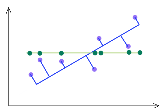
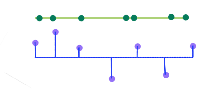
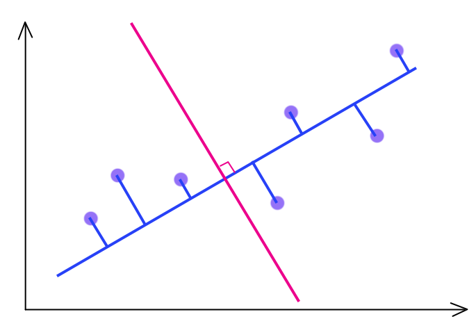
\[\begin{split} G & = G_{1} z_1 + G_{2} z_2 + G_{3} z_3 + G_{4} z_4 \\ \end{split}\]For d = 2 and k = 1, 2D features (purple dots) are projected onto the 1D blue line.
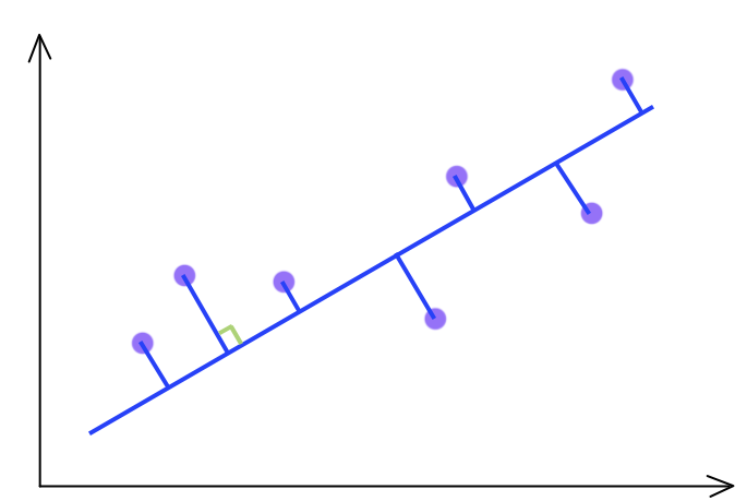
PCA selects a projection that can maximize the variance of their output. Hence, PCA will pick the blue line over the green line if it has a higher variance.
Matrix factorization
PCA can formulated as an approximation to the matrix factorization.
\[\text{X: N x d} \\ \text{Z: N x k} \\ \text{W: k x d} \\\] \[X \approx Z W \\\]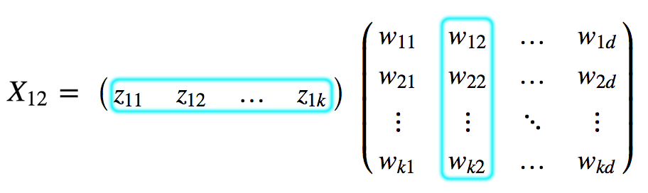
PCA Cost Function
We want to minimize the MSE for \(x\) and the corresponding value for the latent variable \(z\). \((\hat{x} = w^T_j z_i)\):
\[\begin{split} J(W, Z) & = \sum^N_{i=1} \sum^d_{j=1} (w^T_j z_i - x_{ij})^2 \\ & = \sum^N_{i=1} \| W^T z_i - Xi \|^2 \\ & = \| ZW - X \|^2_F \\ \end{split}\]which
\[\| M \|^2_F = \sum_i \sum_j m_{ij}^2\]Solving W
First, we need to perform feature scaling on input features \(x_i\):
\[\begin{split} x^i_j = \frac{x^i_j - \mu_j }{\sigma_j} \end{split}\]\(x^i\) is the ith training datapoints.
which \(\mu_j \text{ and } \sigma_j\) are the mean and standard deviation for the feature \(x_i\). For an image, they are the means and standard deviations of each pixel. For a 100x100x3 image, we will have 30,000 \(\mu_j \text{ and } \sigma_j\).
PCA is based on unsupervised learning. We want to optimize the latent factors \(W\) and latent variables \(Z\) for the cost function \(J\)
\[\begin{split} J(W, Z) & = \| ZW - X \|^2_F \\ \end{split}\]Gradient descent
One of the method to solve PCA is to use Gradient descent to optimize the trainable parameters \(W\) and \(Z\) with the cost function above.
Alternating minimization:
Alternating minimization is another method to find a solution for PCA.
- Optimize ‘W’ with ‘Z’ fixed
- Optimize ‘Z’ with ‘W’ fixed
- Keep repeating
Singular value decomposition (SVD)
Both methods above solve the PCA using empirical method. SVD solves the PCA analytically. Before discussing it in details, we discuss the Singular value decomposition first (SVD). SVD decompose a matrix into 3 matrice as:
\[\begin{split} A_{nxp} & = U_{nxn} S_{nxp} V^T_{pxp} \quad \quad \text{where } U^TU & = I, V^TV = I \\ \end{split}\]The matrix \(U\) and \(V\) is later used to transfrom \(x\) to \(z\) in PCA.
SVD consists of
- Finding the eigenvalues and eigenvectors of \(AA^T\) and \(A^TA\)
- The eigenvectors of \(AA^T\) make up the columns of U
- The eigenvectors of \(A^TA\) make up the columns of V
- The singular values in S are square roots of eigenvalues from \(AA^T\) or \(A^TA\)
Let’s go through an example:
\[A = \begin{bmatrix} 2 & 4 \\ 1 & 3 \\ 0 & 0 \\ 0 & 0 \\ \end{bmatrix}\] \[A A^T = \begin{bmatrix} 2 & 4 \\ 1 & 3 \\ 0 & 0 \\ 0 & 0 \\ \end{bmatrix} \begin{bmatrix} 2 & 1 & 0 & 0\\ 4 & 3 & 0 & 0 \\ \end{bmatrix} = \begin{bmatrix} 20 & 14 & 0 & 0\\ 14 & 10 & 0 & 0 \\ 0 & 0 & 0 & 0 \\ 0 & 0 & 0 & 0 \\ \end{bmatrix} = B\]The eigenvector \(X\) and eigenvalue \(\lambda\) of \(A\) is defined as:
\[\begin{split} Bx & = \lambda x \quad \quad \text{which } \lambda \text{ is a scalar.} \\ (B - \lambda I ) x & = 0 \\ \end{split}\]Now solving:
\[\begin{split} det \begin{bmatrix} 20 - \lambda & 14 & 0 & 0\\ 14 & 10- \lambda & 0 & 0 \\ 0 & 0 & - \lambda & 0 \\ 0 & 0 & 0 & - \lambda \\ \end{bmatrix} = 0 \end{split}\]The eigenvalues are:
\[\lambda_1 \approx 29.88 \\ \lambda_2 \approx 0.118 \\ \lambda_3 = 0 \\ \lambda_4 = 0 \\\]We always sort lambda in the descending order. The kth highest eigenvectors will be used for \(W\).
For \(\lambda_1 = 29.88\)
\[\begin{split} \begin{bmatrix} 20 - 29.88 & 14 & 0 & 0\\ 14 & 10 - 29.88 & 0 & 0 \\ 0 & 0 & 0 & 0 \\ 0 & 0 & 0 & 0 \\ \end{bmatrix} \cdot x & = 0 \\ \implies -9.883 x_1 + 14 x_2 & = 0 \\ 14 x_1 - 19.88 x_2 & = 0 \\ \end{split}\] \[\begin{split} \begin{bmatrix} x_1 \\ x_2 \\ x_3 \\ x_4 \\ \end{bmatrix} & = \begin{bmatrix} 0.82\\ 0.58\\ 0\\ 0\\ \end{bmatrix} \end{split}\]which is the first column of \(U\).
For \(\lambda_2 = 0.118\)
\[\begin{split} 19.883 x1 + 14 x2 = 0 \\ 14 x1 + 9.883 x2 = 0 \end{split}\] \[\begin{split} \begin{bmatrix} x_1 \\ x_2 \\ x_3 \\ x_4 \\ \end{bmatrix} & = \begin{bmatrix} -0.58\\ 0.82\\ 0\\ 0\\ \end{bmatrix} \end{split}\]which is the second column of \(U\).
We can skip all the eigenvalues = 0. Hence:
\[\begin{split} U = \begin{bmatrix} 0.82 & -0.58& 0 & 0\\ 0.58 & 0.82& 0 & 0\\ 0 & 0 & 1 & 0\\ 0 & 0 & 0 & 1\\ \end{bmatrix} \end{split}\]Similarly, we calculate \(A^TA\) to find \(V\) which is:
\[\begin{split} V = \begin{bmatrix} 0.4 & -0.91\\ 0.91 & 0.4\\ \end{bmatrix} \end{split}\]The singular values in S are square roots of eigenvalues from \(AA^T\) or \(A^TA\):
\[\begin{split} S = \begin{bmatrix} \sqrt{29.88} = 5.47 & 0 \\ 0 & \sqrt{0.12} = 0.37\\ 0 & 0 \\ 0 & 0 \\ \end{bmatrix} \end{split}\]The sample above is originated from [http://web.mit.edu/be.400/www/SVD/Singular_Value_Decomposition.htm]
Now we apply SVD to solve PCA. First we compute the covariance matrix with our \(m\) n-Dimensional training datapoints \(x\).
\[\Sigma = \frac{1}{m} \sum^M_{i=1} x^i (x^i)^T\]\(\Sigma\) is a nxn matrix
\[\begin{split} \Sigma_{nxn} = x_{nx1} \cdot (x)^T_{1xn} \end{split}\]Apply SVD to decompose \(\Sigma\) to \(U\):
\[\begin{split} \Sigma_{nxn} & = U_{nxn} S_{nxn} V^T_{nxn} \\ \Sigma & = U S V^T \\ \end{split}\]Which \(U\) have the dimension of:
\[U = \begin{bmatrix} u_{11} & u_{12} & \cdots & u_{1k} \cdots u_{1n}\\ u_{21} & u_{22} & \cdots & u_{2k} \cdots u_{2n}\\ \vdots & \vdots & \ddots & \vdots \\ u_{n1} & u_{n2} & \cdots & u_{nk} \cdots u_{nn}\\ \end{bmatrix}\]We only take the first k columns:
\[U = \begin{bmatrix} u_{11} & u_{12} & \cdots & u_{1k} \\ u_{21} & u_{22} & \cdots & u_{2k} \\ \vdots & \ddots & \vdots \\ u_{n1} & u_{n2} & \cdots & u_{nk} \\ \end{bmatrix}\]To transform \(X\) to \(Z\):
\[z = U^T x\]Let’s check the dimensionality again:
\[z_{kx1} = (U^T)_{kxn} x_{nx1}\]To convert \(z\) to \(x\):
\[x = U z\]Predicting Z
Given \(W\) and testing data \(\hat{X}\), \(\hat{Z}\) is computed by first subtract the training mean from the features and then calculate \(Z\).
\[\begin{split} \hat{x}^i & = \hat{x}^i -\mu \\ \hat{Z} & = \hat{X}W^T(WW^T)^{-1} \\ \end{split}\]Choosing the number of latent factors k
PCA is about maximizing variance. Say to keep 90% of variance, we set \(R = 0.1\).
\[\begin{split} J_k & = \| ZW - X \|^2_F \\ J_0 & = \| X \|^2_F \\ \\ \frac{J_k}{J_0} & = \frac{\| ZW - X \|^2_F}{\| X \|^2_F} < R \\ R & > \frac{\| ZW - X \|^2_F}{n \cdot var(x_{ij})} \end{split}\]Alternatively, we can start from k=1 and increment it until say \(T \lt 0.01\).
\[\Sigma = \frac{1}{m} \frac{\sum^M_{i=1} \| x^i - (\hat{x})^i \|^2} {\sum^M_{i=1} \| x^i \|^2 } \lt T = 0.01\]\(S\) stores the eigenvalues of the eigenvectors but also reflect how important for a particular latent factors. Hence, we can also determine k by:
\[\begin{split} S = \begin{bmatrix} S_{11} & 0 & 0 & \cdots & 0 \\ 0 & S_{22} & 0 & \cdots & 0 \\ 0 & 0 & S_{33} & \cdots & 0 \\ \vdots & \ddots & \vdots \\ \end{bmatrix} \end{split}\] \[\frac{\sum^k_{i=1} S_{ii}}{\sum^n_{i=1} S_{ii}} \gt T = 0.99\]W uniqueness (orthogonal)
The solution for W is not unique. But we can impose a few restrictions to solve this.
- Set the magnitude of the principal component to 1. (\(W_{c_i}\): row \(c_i\) of \(w\))
- Each latent factors are independent of each other (cross product = 0).
We can still have the factors \(W_{c_i}\) rotated or label switching \(W_{c_i}\) switch to \(W_{c_i^{'}}\). To fix this, we can
- First set k = 1, and solve W with the constraint above
- Set k = 2 with the first factor set and solve \(W\) for the second factor \(W_2\)
- Repeat until reaching our target k
The blue line is our first optimized W for \(k = 1\). The optimal solution \(W\) for \(k = 2\) is the red line orthogonal to the blue line.
With these constraints:
\[\begin{split} \| w_{c_i} \| & = 1 \\ w_{c_i}^T w_{c_i^{'}} & = \begin{cases} 1 \quad \text{ if } c_i = c_i^{'} \\ 0 \quad \text{ if } {c_i} \neq c_i^{'} \\ \end{cases} \\ \\ \implies W W^T & = I \\ \end{split}\]Solving Z becomes:
\[\begin{split} Z & = XW^T(WW^T)^{-1} \\ & = XW^T \end{split}\]Eigenfaces
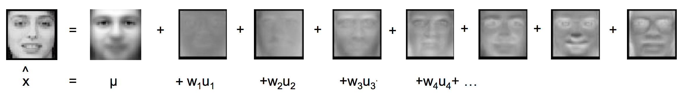
Eigenfaces apply PCA to represent a facial image with latent factors. First we compute the mean image and the top k eigenvectors (Principal components)
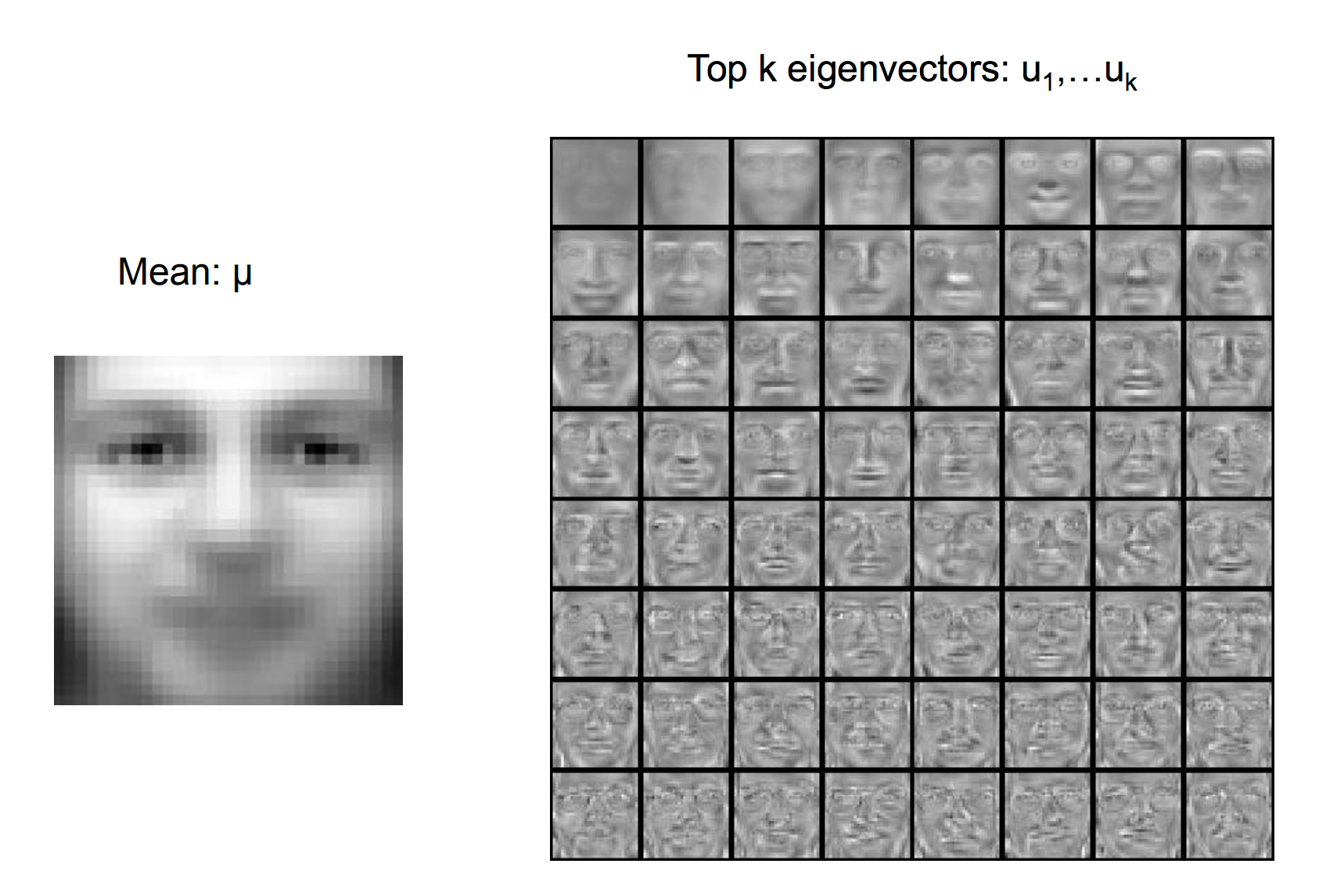
The image is encoded with the latent factors:
Non-negative matrix factorization (NMF):
NMP is similar to the matrix factorization methods above with the same cost functions, except that we add an additional constraint that \(W\) and \(Z\) are non-negative.
IN NMF,
- \(W\) and \(Z\) are non-negative instead of orthogonal
- Promote sparsity
- Avoiding postive & negative matrix elements cancelling each other
- Brain seem to use sparse representation
- Energy efficient
- Increase the number of concepts that can memorize
- Learning the parts of objects
In NMF. the latent factors are more close to individual facial features.
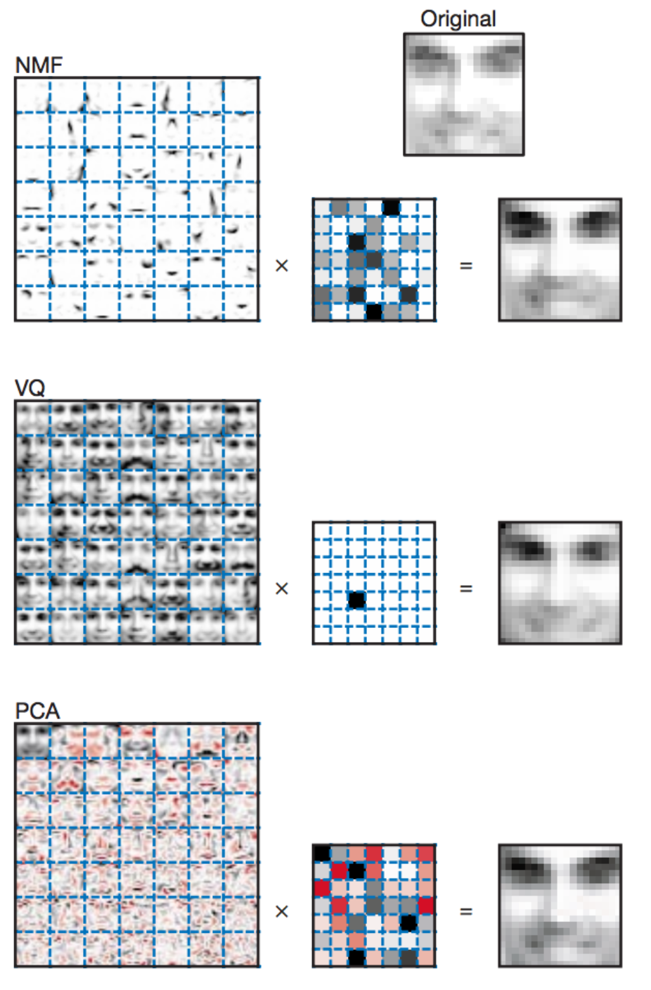
Credit: Daniel D. Lee: Learning the parts of objects by non-negative matrix factorization
Sparse Matrix Factorization
Sparse Matrix Factorization promotes the sparsity of \(W\).
Here is the plot of J with an optimized \(w\) smaller than 0.
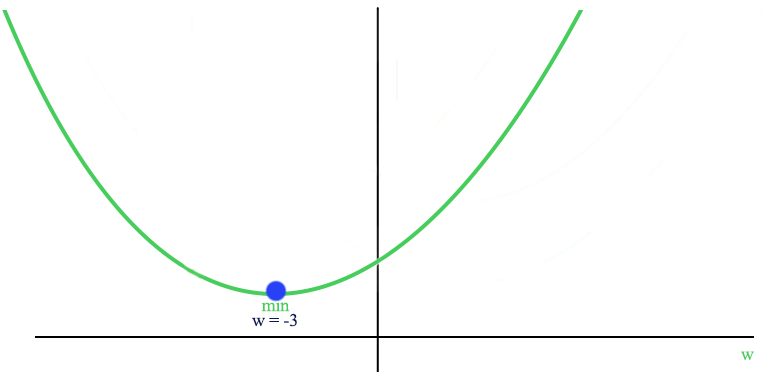
With the constraint of \(w>0\), the optimized cost is now at \(w=0\) (promote sparsity).
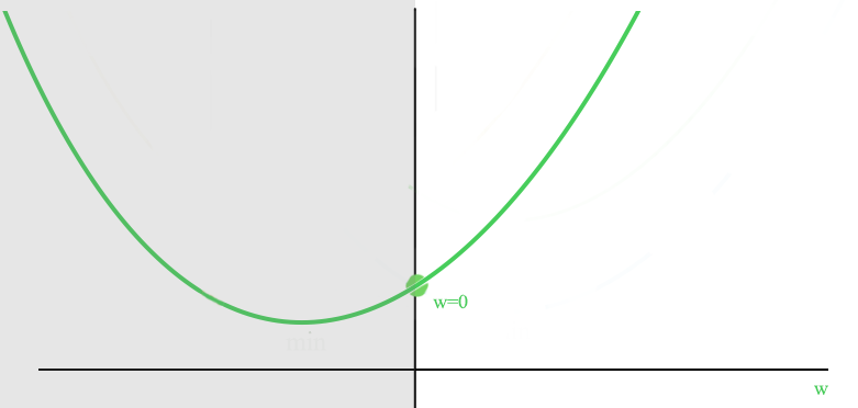
We are going to use Gradient descent to train \(W\) and reset the value to 0 if it is negative:
\[w_i = max(0, w_i - \alpha \nabla_{w_i} J)\]L1-regularization
We can also use L1 regularization to control sparsity:
\[\begin{split} J(W, Z) & = \| ZW - X \|^2_F + \frac{\lambda_1}{2} \| W \|_1 + \frac{\lambda_2}{2} \| Z \|_1 \\ \end{split}\]Here is the visualization of latent factors with different techniques:
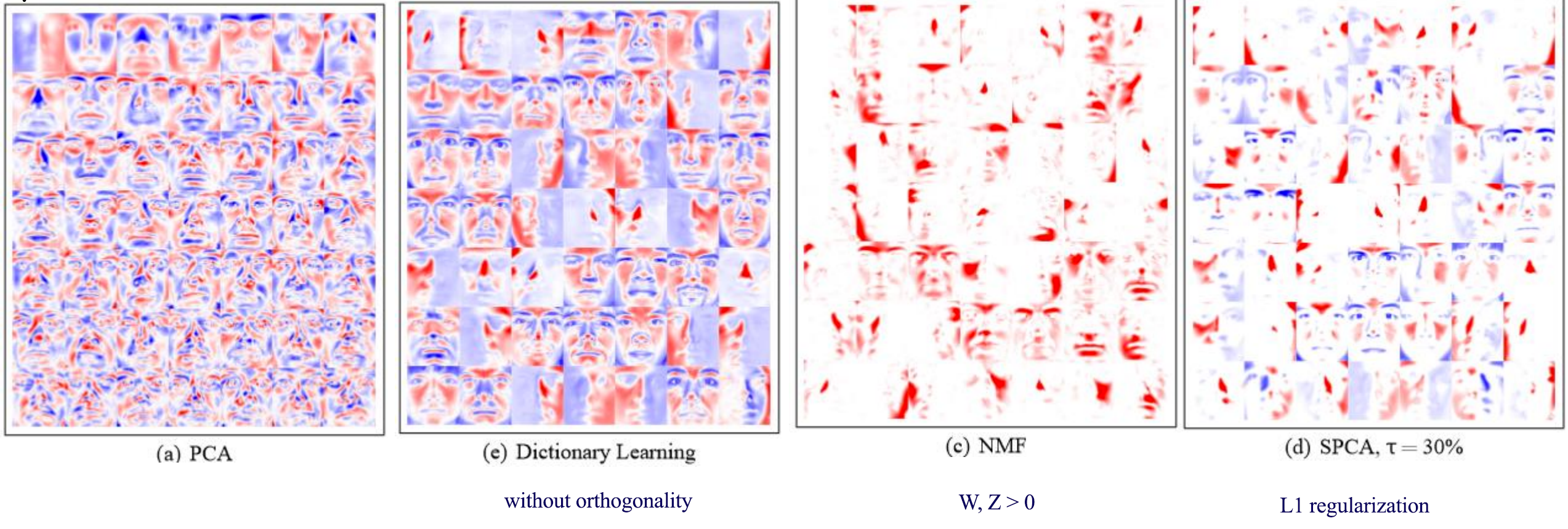
Credit: Julien Mairal etc… Online Learning for Matrix Factorization and Sparse Coding
Regularized Matrix Factorization
Instead of forcing orthogonality, we can add a L2 regularization cost to control how \(W\) is optimized.
\[\begin{split} J(W, Z) & = \| ZW - X \|^2_F + \frac{\lambda_1}{2} \| W \|^2_f + \frac{\lambda_2}{2} \| Z \|^2_f \\ \end{split}\]Latent Factor Model using logistic loss
We can also use logistic loss for our cost function
\[\begin{split} J(W, Z) & = \sum^n_{i=1} \sum^d_{j=1} \log( 1+ e^{ - x_{ij}w^T_jz_i} ) \end{split}\]Robust PCA
To reduce the effects of outlier, Robust PCA switch to a L1-norm in calculating the errors.
\[\begin{split} J(W, Z) & = \vert ZW - X \vert \\ \end{split}\]