“Machine learning - Anomaly detection”
Anomaly detection
Model-based outlier detection
Z-score measures the probability of \(x_i\):
\[Z_i = \frac{X_i - \mu}{\sigma}\]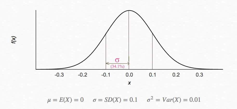
Issue: The outlines contributes to the value of \(\mu\) and \(\sigma\) and assume it is uni-modal. (The probability distribution function has only 1 peak.)
The Gaussian probability distribution is
\[p(x) = \frac{1}{\sigma\sqrt{2\pi}}e^{-(x - \mu)^{2}/2\sigma^{2} }\]- Locate features that indicate anomaly behavior
- Collect training dataset
- Calculate \(\mu_i\) and \(\sigma_i\) for every feature \(x_i\)
- For a new testing data \(x = (x_1, x_2, \cdots, x_n)\), compute the probability
- Flag the data if
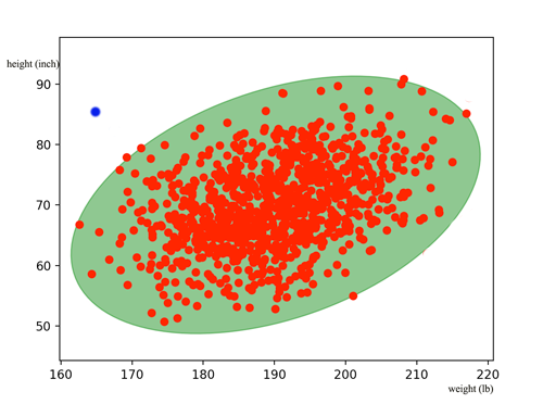
However, features in \(x\) may be co-related. The diagram below shows weight and height are co-related. The green zone are datapoints consider as normal. The blue dot falls within the normal height or weight of the population. But knowing the person is much taller but yet much ligher, we should flag this data as abnormal. Nevertheless, the equation above does not account for the co-relationship between variables.
To compensate that, we should not compute \(p(x_i; \mu_j, \sigma^2_i)\) individually as in
\[p(x) = \prod^n_{i=1} p(x_i; \mu_j, \sigma^2_i)\]Instead we need to compute the probability using a multivariate Gaussian distribution. The covariance matrix \(\Sigma\) will compensate any co-relationship between features and make the necessary adjustments.
\[P(x ) = \frac{1}{\sqrt{(2\pi)^n \vert \Sigma \vert}}e^{- \frac{1}{2}(x - \mu)^T \Sigma^{-1} (x - \mu)} \\\] \[\Sigma = \begin{pmatrix} E[(x_{1} - \mu_{1})(x_{1} - \mu_{1})] & E[(x_{1} - \mu_{1})(x_{2} - \mu_{2})] & \dots & E[(x_{1} - \mu_{1})(x_{p} - \mu_{p})] \\ E[(x_{2} - \mu_{2})(x_{1} - \mu_{1})] & E[(x_{2} - \mu_{2})(x_{2} - \mu_{2})] & \dots & E[(x_{2} - \mu_{2})(x_{p} - \mu_{p})] \\ \vdots & \vdots & \ddots & \vdots \\ E[(x_{p} - \mu_{p})(x_{1} - \mu_{1})] & E[(x_{p} - \mu_{p})(x_{2} - \mu_{2})] & \dots & E[(x_{n} - \mu_{p})(x_{p} - \mu_{p})] \end{pmatrix}\]which \(E\) is the expected value function.
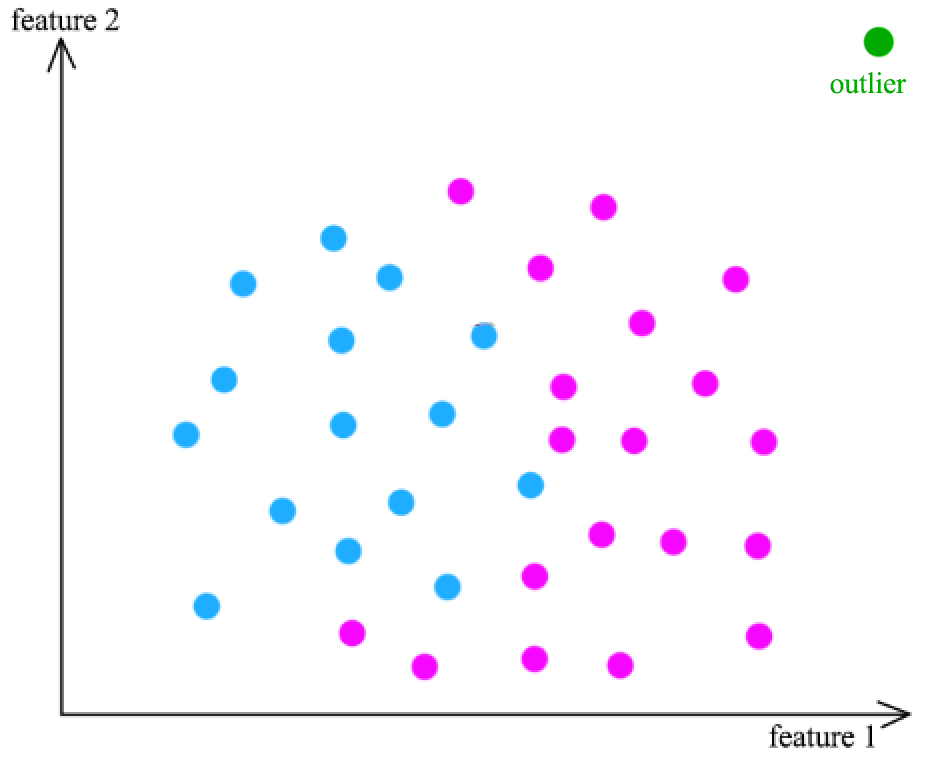
Graphical outlier detection
Plot data to locate outliner visually:
- Use Box plot for 1 variable at a time
- Scattering plot for 2 variables at a time
- Scattering array to look at multiple combination at a time. But still ploting 2 variables at a time
- Scattering plot of 2-D PCA
Cluster-Based outlier detection
- Cluster the data
- Find points that do not belong to a cluster, (density based clustering) or
- Far away from the center of the cluster, (K-medians) or
- Only join a hierarchy clustering at the coarse grain level
Global distance-based outlier detection: KNN
We can measure the distance of a datapoint from its neighbors to detect outliner.
- Calculate the average distance for its K-neighbors
- Choose the biggest values as outliners
- Good for locate global outlier
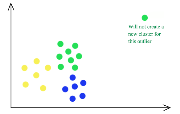
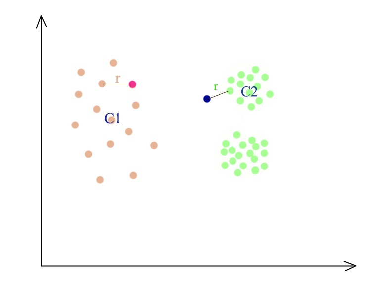
Outlier-ness
Nevertheless, some datapoints may be close to a cluster in the global sense but should not be consider as part of it after consider the average distance among the cluster’s members. Members in the Cluster C2 is closer together than Cluster C1. So even the blue dot is only \(r\) away from the green dot, it is not consider as part of the cluster C2 while the red dot will be consider as part of C1.
The average distance for \(x_i\) from its k neighbors is:
\[\begin{split} D^k(x^i) & = \frac{1}{k} \sum_{j \in N_i} \| x^i - x^j \| \\ \end{split}\]To consider whether it is outlier, we need to consider how close \(x_i\) to its neighbors \(N_i\) and how close those neighbors \(x_l\) are with their neighbors \(N_l\).
\[\begin{split} O^k(x^i) & = \frac{D^k(x^i)}{\frac{1}{k} \sum_{l \in N_j} D^k(x^l)} \end{split}\]If \(O^k(x^i) > 1\), the datapoint between itself and the cluster is greater than the average distance among the cluster members.
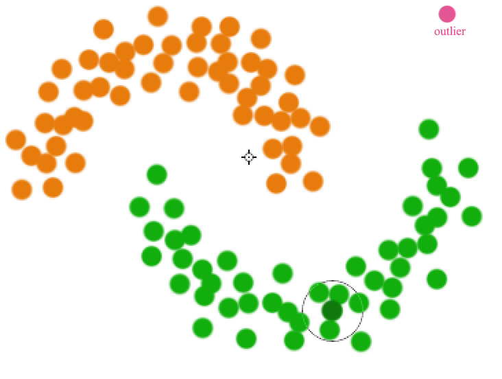
Influenced outlierness
However, we may still have problems for clusters that are very close. The circled green dot has high \(O^k(x^i)\) even though it is part of the green cluster because it counts the red dots as its closest neighbors.
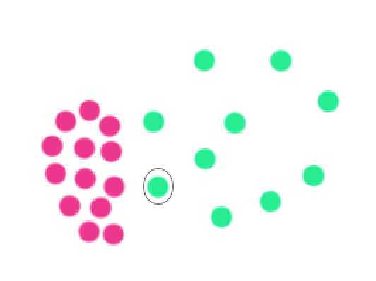
In influenced outlierness, we are not finding the average distance of its neighbors’ neighbors. Instead, we find the average distance of its neighbors that consider \(x_i\) as its neighbors.

Then we replace the denominator with the average distance of those tick dots.
\[\begin{split} O^k(x^i) & = \frac{D^k(x^i)}{\frac{1}{k} \sum_{i \in N_l} D^k(x^l)} \end{split}\]Supervised outlier detection
We can use supervising learning to determine whether a datapoint is an outlier. This method can detect complex rule but will require the labeling of the training data.