“Machine learning - Naive bayes classifier, Bayesian inference”
Bayes’ theorem
Bayes’ theorem calculates the conditional probability (Probability of A given B):
\[P(A \vert B) = \frac{P(B \vert A) P(A)}{P(B)}\]Sometimes the result of the Bayes’ theorem can surprise you . Let’s say there is an un-common decease that only 0.1% of the population has it. We develop a test of 99% accuracy for positive and negative result. What is the chance that you have this decease if your test is positive. The answer is only 9% which is much smaller than you may think. The intuition is that even the test looks accurate, it generates more false positive than true positive because the decease is not common. With Bayes’ theorem, we can demonstrate why it is only 9%.
Notation: \(d\) stands for having the decease and \(+\) stands for testing positive. \(\neg d\) means not d.
\[\begin{equation} \begin{split} P( d \vert + ) &= \frac{P(+ \vert d) P(d)}{P(+)} \\ \\ &= \frac{P(+ \vert d) P(d)}{P(+, d) + P(+, \neg d)} \\ \\ &= \frac{P(+ \vert d) P(d)}{P(+ \vert d)P(d) + P(+ \vert \neg d)P(\neg d)} \\ \\ & = \frac{0.99 * 0.001}{0.99*0.001 + 0.01 *0.999} \\ \\ & = 0.0902 \\ \end{split} \end{equation}\]Convention: \(P(x)\) means \(P(X = x)\). \(P(A, B)\) stand for \(P(A \text{ and } B)\).
Proof of the Bayes theorem:
\[\begin{equation} \begin{split} P(A,B) & = P(A \vert B) P(B) \\ \\ P(A \vert B) & = \frac{P(A,B)}{P(B)}, \quad P(B \vert A) & = \frac{P(A,B)}{P(A)} \\ \\ \frac{P(A \vert B)}{P(B \vert A)} &= \frac{P(A)}{P(B)} \\ \\ P(A \vert B) &= \frac{P(B \vert A) P(A)}{P(B)} \end{split} \end{equation}\]Naive Bayes Classifier
Naive Bayes Classifier classifies objects \(Y\) given observation \(x_1, x_2, \dots, x_n\) based on Bayes’ theorem. For example, if we draw an object from a basket, if it is red and round \((x)\), what is the chance that it is an apple \((Y)\)?
\[\begin{equation} \begin{split} P(Y \vert x_1, x_2, \dots, x_n) & = \frac{P(x_1, x_2, \dots, x_n \vert Y) P(Y)}{P(x_1, x_2, \dots, x_n)} \end{split} \end{equation}\]Assume \({x_i}\) and \({x_j}\) are independent of each others given \(Y\). (An red object does not increase the chance that it is round.) i.e.: \(P(x_1, x_2, \dots \vert Y) = P(x_1 \vert Y) P(x_2 \vert Y) \dots\)
\[\begin{equation} \begin{split} P(Y \vert x_1, x_2, \dots, x_n) & = \frac{P(x_1 \vert Y) P(x_2 \vert Y) ... P( x_n \vert Y) P(Y)}{P(x_1, x_2, \dots, x_n)} \\ \\ & = \frac{P(Y) \prod^n_{i=1} P( x_i \vert Y) }{P(x_1, x_2, \dots, x_n)} \\ \\ & \propto P(Y) \prod^n_{i=1} P( x_i \vert Y) \end{split} \end{equation}\]Example
Let’s say we want to determine whether an object we pick in a basket is an apple or a grape given the object is red, round & sweet
\[\begin{equation} \begin{split} P(apple \vert red, round, sweet) & = \frac{P(red, round, sweet \vert apple) P(apple)}{P(red, round, sweet)} \\ \\ & = \frac{P(red | apple) P(round | apple) P(sweet | apple ) P(apple)}{P(red, round, sweet)} \\ \end{split} \end{equation}\]\(P(red, round, sweet)\) is the same regardless of which object to pick, therefore we ignore the denominator in comparing object’s probability. \begin{equation} \begin{split} P(apple \vert red, round, sweet) & \propto P(red | apple) P(round | apple) P(sweet | apple ) P(apple) \end{split} \end{equation}
Say, half of the object in the basket are apples, and
\[\text{Given: } P(red \vert apple) = 0.7, P(round \vert apple) = 0.98, P(sweet \vert apple) = 0.9\]The chance that the object is an apple:
\[P(apple \vert red, round, sweet) \propto 0.7 \cdot 0.98 \cdot 0.9 \cdot 0.5 = 0.6174\]If a quarter of the object in the basket are grapes, the corresponding chance for a grape is:
\[\text{Given: } P(red \vert grape) = 0.6, P(round \vert grape) = 0.95, P(sweet \vert grape) = 0.3\] \[P(grape \vert red, round, sweet) \propto 0.6 \cdot 0.95 \cdot 0.3 \cdot 0.25 = 0.04\]So if an object is red, round and sweet, it is likely an apple.
E-mail spam filter
We use bag of words to construct features \(x_i\).
| money | inheritance | rich | quick | vicodin | free | fee | bank | illegal | alcohol | … | |
| Message | 1 | 0 | 1 | 0 | 0 | 0 | 1 | 0 | 0 | 1 | … |
If p(yi = ‘spam’ | xi) > p(yi = ‘not spam’ | xi),
	classify as spam
Tips:
To avoid
\[P(word \vert spam) = 0\]We count \(P(word \vert spam)\) as
\[\frac{(n_{word} + β)}{(n + 2β)}\]To avoid underflow in multiple small numbers, we take the logarithm of the equation which turns those probability multiplication into additional.
People may be more tolerance on false negative than false positive in classify e-mail as spam. So, instead of comparing the
\[p(spam \vert x_i) > p(\neg spam \vert x_i)\]We give a weight in the comparison
\[p(spam \vert x_i) > w \cdot p(\neg spam \vert x_i) \text{ which } w >1\]Bayesian inference
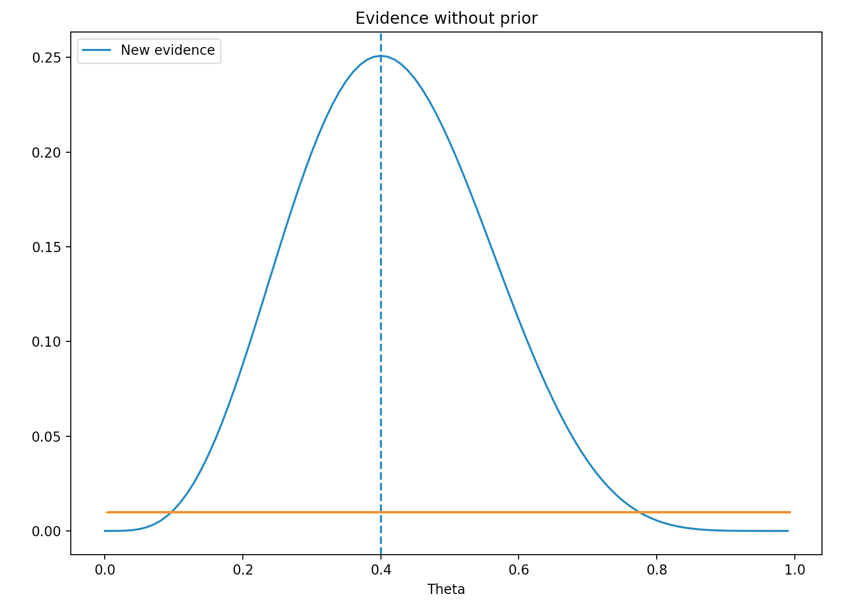
Let’s go through an example in determine the infection rate (\(\theta\)) for Flu. On the first day of the month, we got 10 Flu testing results back. We call this evidence \((x)\). For example, our new evidence shows that 4 samples are positive. \((x=4 \text{ out of 10})\). We can conclude that (\(\theta = 4/10 = 0.4\)). Nevertheless we want to study further by calculating the probability of \(x\) given a specific \(\theta\).
The chance of \(x\) given \(\theta\) is the likelihood of our evidence. In simple term, likelihood is how likely the evidence (4 samples are positive) will happen (or generated) with different infection rate. Based on simple probability theory:
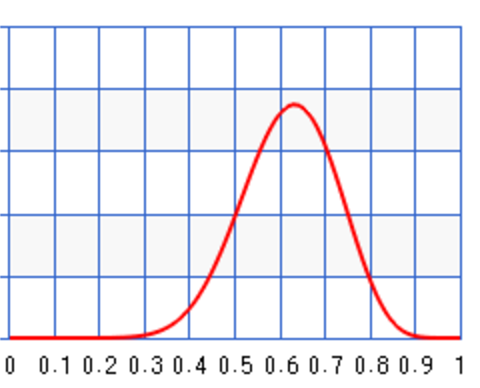
\[\begin{align} P(x \vert \theta) &= {n \choose x} \theta^x(1-\theta)^{n-x}\\ &= \dfrac{10!}{4!(10-4)!}\theta^4 (1-\theta)^{10-4}\\ \end{align}\]We plot the probability for values \(\theta\) range from 0 to 1. Maximum likelihood estimation (MLE) is where \(\theta\) has the highest probability. Here MLE is 0.4. i.e. the most likely value for \(\theta\) with the evidence \(x\) is 0.4.
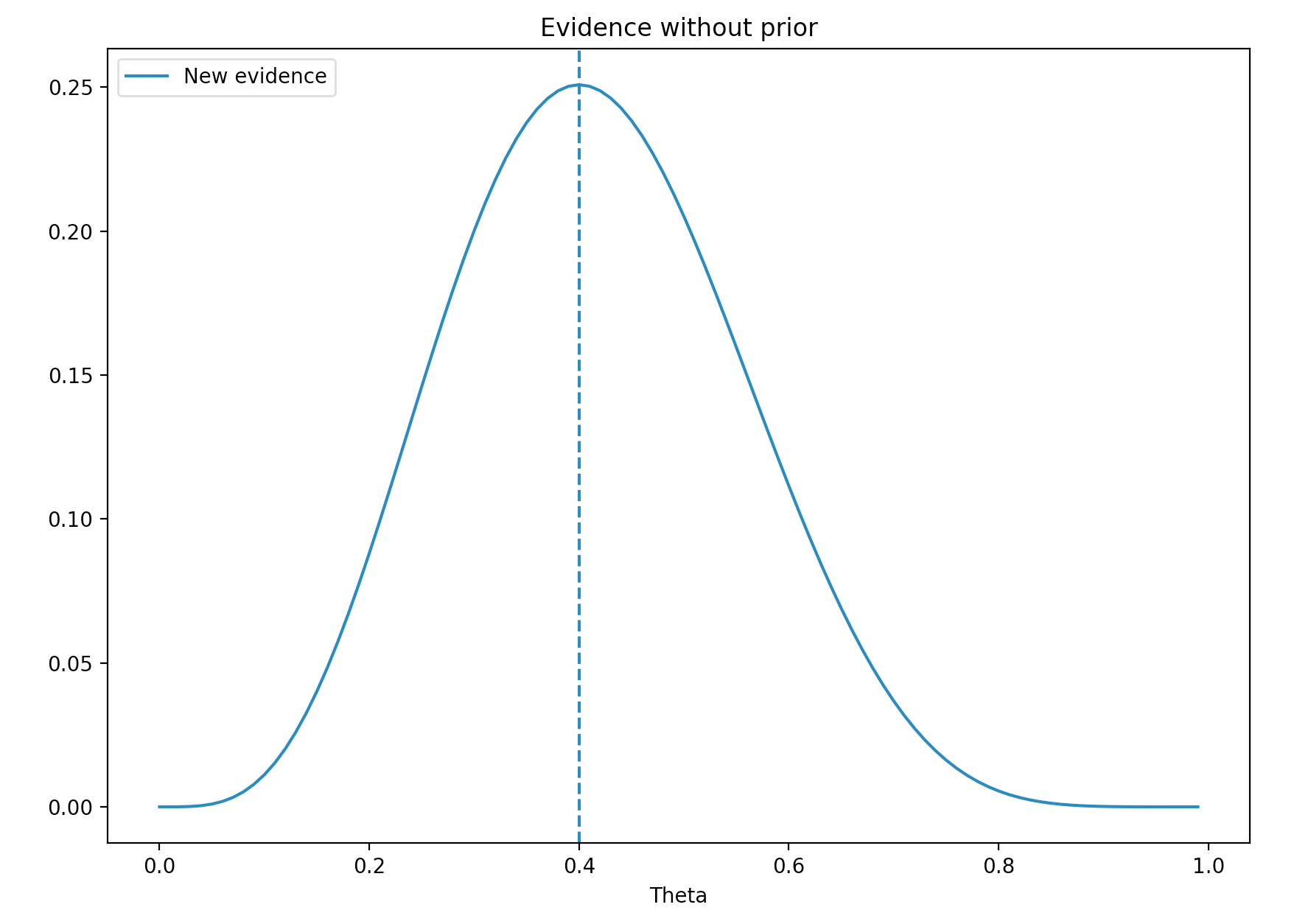
We called \(P(x \vert \theta)\) the likelihood. The blue line above is the likelihood.
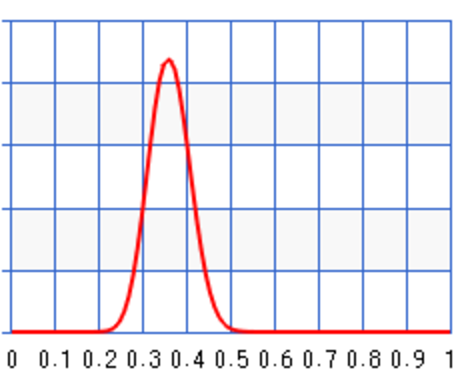
In a stochastic process, the computed value is not a scalar but a probability distribution. We may predict \(\theta\) has a mean value of 0.3 with a variance 0.1. If we need a scalar value, we sample it from the probability distribution.
We had also collected 100 months of data on the infection rate for flu. This data forms a belief of the Flu infection rate which we usually call prior \(P(\theta)\). The orange line below is \(P(\theta)\). It is the prior belief of the probability distribution for \(\theta\). The distribution centers around 0.14 meaning we generally believe the average infection rate of Flu is 0.14. The blue line is the probability distribution of \(\theta\) just based on the new evidence. (likelihood) Obviously the new evidence is different from the prior (belief).
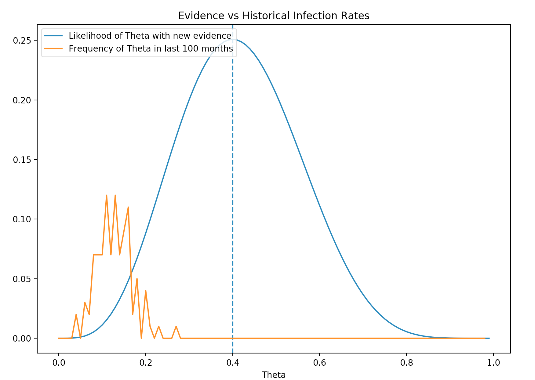
We either suspect that the much higher infection rate of the new evidence is caused by low sampling size of the new evidence or we encounter a new strength of Flu that we need to re-adjust the prior.
Recap the terminology
\[P(H \vert E) = \frac{P(E \vert H) P(H)}{P(E)}\]People discuss Bayes with a lot of terminologies. We pause a while to summarize the terms again.
Evidence E (observation) is some data we observed . For example, 4 tests out of the 10 collected test positive. We can treat belief H as a hypothesis. For example, we can start with a belief of 0.14 infection rate with a variance 0.02 and later use Bayes inference to refine it with data that we collect.
| posterior probability | \(P(H \vert E)\) | The refined belief given the new observed evidence. The new belief after merging prior belief with the evidence. |
| likelihood | The probability of the evidence given the belief. The chance of have 4 positive samples out of 10 for different infection rates. |
|
| prior | The probability of the belief prior to new evidence. This is likely from some prior knowledge or experience. |
|
| marginal probability | The probability \(\sum_x P(E, H)\) for all possible infection rates. The probability of seeing 4 positive samples under all possible infection rates . |
Bayesian inference (continue)
Bayesian inference try to draw better prediction based on evidence and prior belief.
With Bayes inference, we calculate the posterior probability \(P(\theta \vert x)\) using Bayes theory. We re-calibrate our belief given the new evidence:
\[P(\theta \vert x) = \frac{P(x \vert \theta) P(\theta)}{P(x)}\]Here is the plot of the posterior. The yellow line is the prior \(P(\theta)\), the blue line is the likelihood. The green line is the posterior calculated with the Bayes theory.
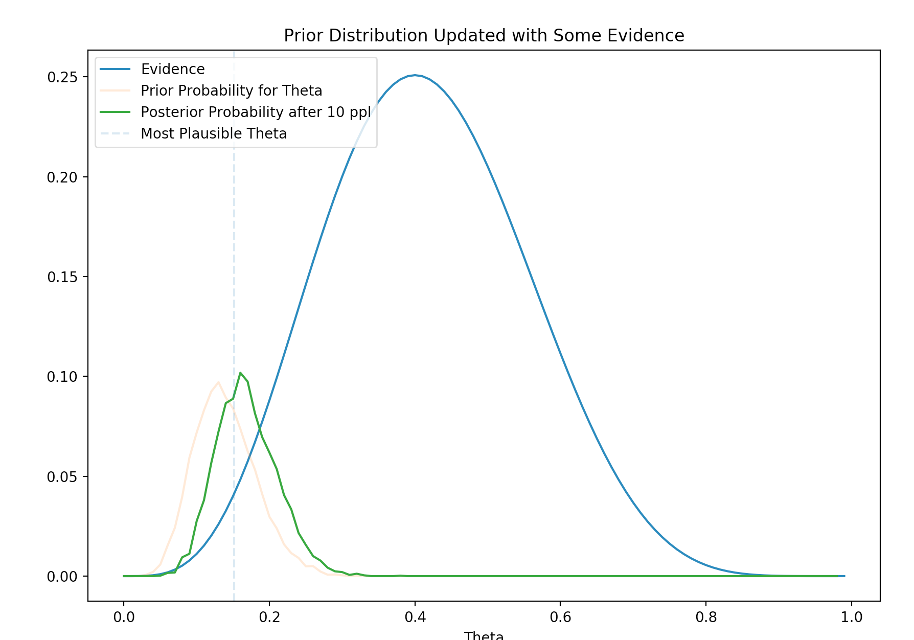
It is clear that the posterior moves closer to the likelihood with the new evidence. The posterior
\[P(\theta \vert x) = \frac{P(x \vert \theta) P(\theta)}{P(x)}\]depends on the prior and the likelihood. Even the prior peaks at 0.14 (the red line). The new evidence has a likelihood that contradict it. The likelihood at the red line is lower and therefore their posterior (their multiplication), shown as the green dot, is lower. At the vertical green line, even the prior is lower but it is compensated by the higher likelihood and therefore the peak of the posterior moves towards the likelihood.
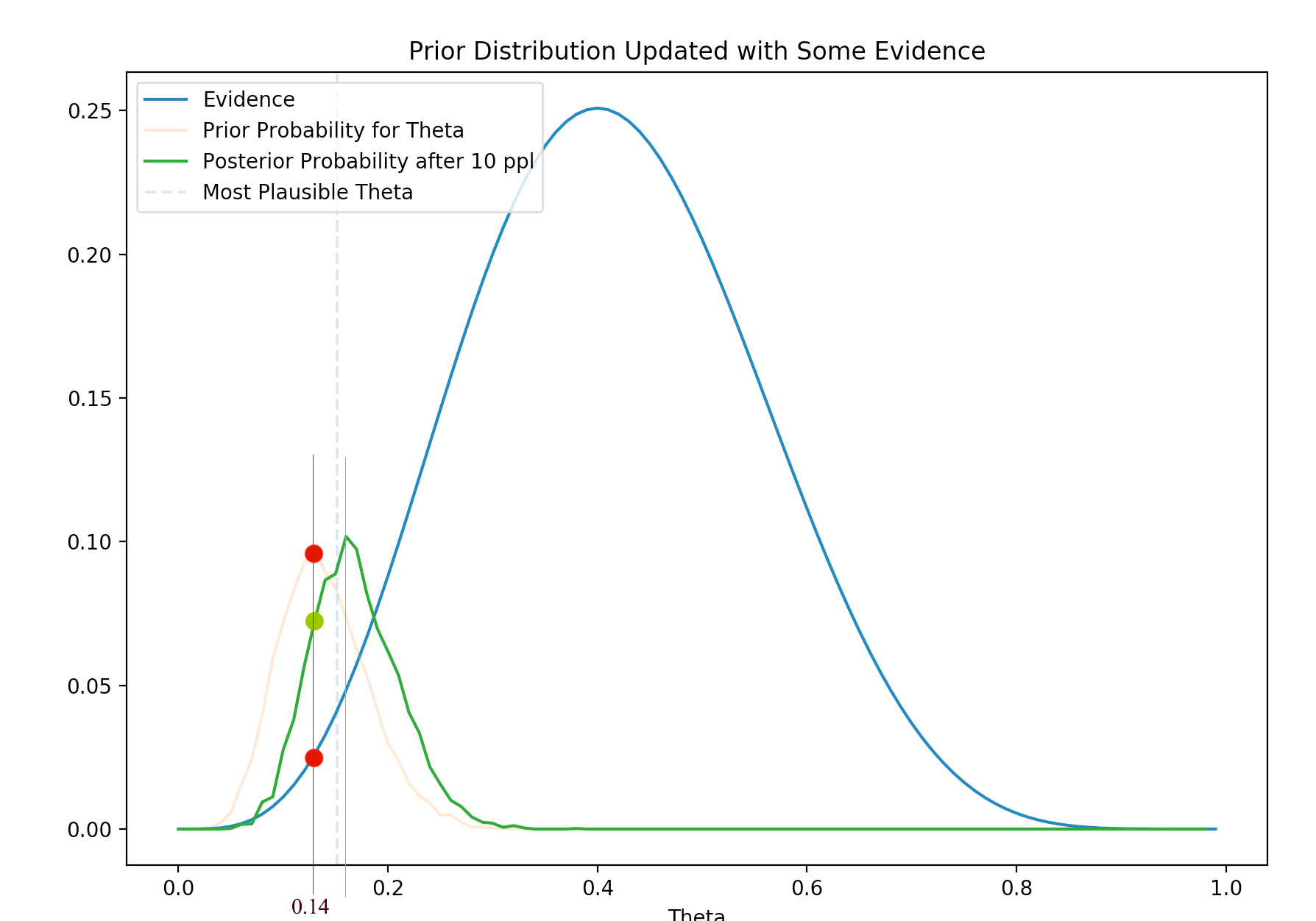
In short, with new evidence, we shift our belief towards the direction of the newly observed data. We re-calibrate the belief with new data.
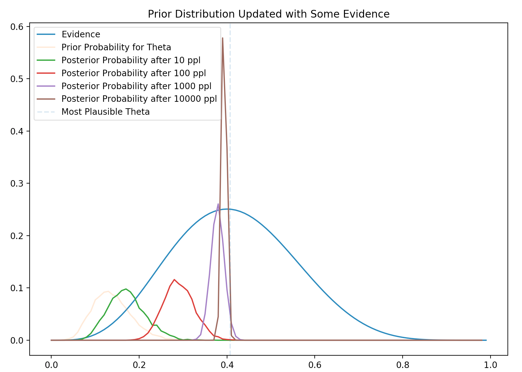
In Bayes inference, we can start with certain belief for the probability distribution of \(\theta\). Alternatively, we can start with a random guess say it is uniformed distributed like the orange line below. e.g. the chance that \(\theta=0.1\) is the same as \(\theta=0.9\). The first calculated posterior with this prior will equal to the likelihood.
With new round of evidence, we compute the new posterior given the evidence. This posterior becomes our belief (prior) in the next iteration when another round of evidence is collected. After many iterations, our prior will converge to the true probability distribution of \(\theta\).
How far the posterior will move towards to the new evidence? It depends on the size of the evidence. Obviously, a large sampling size will move the posterior closer. The following plot indicates that the larger the size of the evidence, the further it moves towards the evidence. The variance decreases also and we are more certain on its value.
Beta distribution for prior
The definition of a beta distribution is:
\[\begin{align} P(\theta \vert a, b) = \frac{\theta^{a-1} (1-\theta)^{b-1}} {B(a, b)} \end{align}\]where \(a\) and \(b\) are parameters for the beta distribution.
For discret variable, the beta function \(B\) is defined as:
\[\begin{align} B(a, b) & = \frac{\Gamma(a) \Gamma(b)} {\Gamma(a + b)} \\ \Gamma(a) & = (a-1)! \end{align}\]For continuos variable, the beta function is:
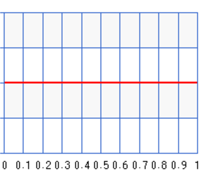
\[\begin{align} B(a, b) = \int^1_0 \theta^{a-1} (1-\theta)^{b-1} d\theta \end{align}\]For our discussion, let \(\theta\) be the infection rate of the flu. With Bayes’ theorem, we study the probabilities of different infection rates rather than just finding the most likely infection rate. The prior \(P(\theta)\) is the belief on the probabilities for different infection rates. \(P(\theta=0.3) = 0.6\) means the probability that the infection rate equals to 0.3 is 0.6. If we know nothing about this flu, we use an uniform probability distribution for \(P(\theta)\) in Bayes’ theorem and assume any infection rate is equally likely.
An uniform distribution maximizes the entropy (randomness) to reflect the highest uncertainty of our belief.
We use Beta function to model our belief. We set \(a=b=1\) in the beta distribution for an uniform probability distribution. The following plots the distribution \(P(\theta)\):
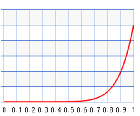
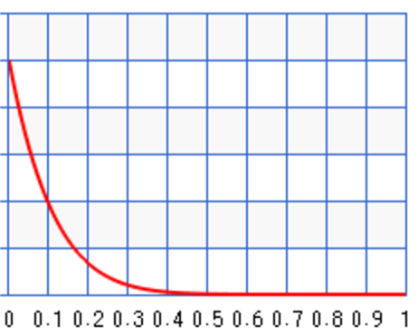
Different values of \(a\) and \(b\) result in different probability distribution. For \(a=10, b=1\), the probability peaks towards \(\theta=1\) :
For \(a=1, b=10\), the probability peaks towards \(\theta=0\):
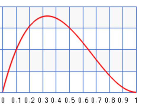
For example, we can start with some prior information about the infection rate of the flu. For example, for \(a=2, b=3\), we set the peak around 0.35:
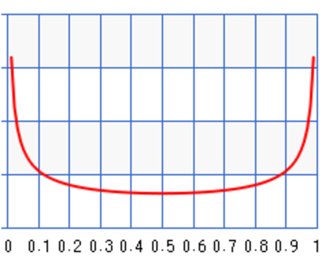
For \(a=b=0.5\):
We model the likeliness \(P(data \vert \theta)\) of our observed data given a specific infection rate with a Binomial distribution. For example, what is the possibility of seeing 4 infections (variable x) out of 10 (N) samples given the infection rate \(\theta\).
\[\begin{align} P(data \vert \theta) & = {N \choose x} \theta^{x} (1-\theta)^{N-x} \end{align}\]Let’s apply the Bayes theorem to calculate the posterior \(P(\theta \vert data)\): the probability distribution function for \(\theta\) given the observed data. We usually remove constant terms from the equations because we can always re-normalize the graph later if needed.
\[\begin{align} P(data \vert \theta) & \propto \theta^x(1-\theta)^{N-x} & \text{ (model with a Binomial distribution) }\\ P(\theta) & \propto \theta^{a-1} (1-\theta)^{b-1} & \text{ (model as a beta distribution) }\\ \end{align}\]Using Bayes’ theorem:
\[\begin{align} P(\theta \vert data) & = \frac{P(data \vert \theta) P(\theta)}{P(data)} \\ & \propto P(data \vert \theta) P(\theta) \\ & \propto \theta^{a + x -1} (1-\theta)^{N + b -x -1} \\ & = B(a+x, N + b - x) \end{align}\]We start with a Beta function for the prior and end with another Beta function as the posterior. Pior is a conjugate prior if the posterior is the same class of function as the prior. As shown below, this helps us to calculate the posterior much easier.
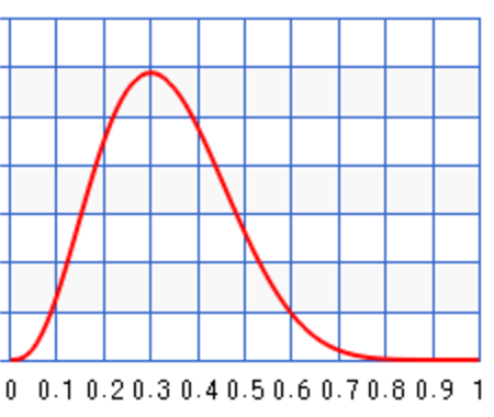
We start with the uniformed distributed prior \(P(\theta) = B(1, 1)\) assuming we have no prior knowledge on the infection rate. \(\theta\) is equally likely for any values between [0, 1].
For the first set of sample, we have 3 infections our of a sample of 10. (\(N=10, x=3\)) The posterior will be \(B(1+3, 10 + 1 - 3) = B(4, 8)\) which has a peak at 0.3. Even assuming no prior knowledge (an uniform distribution), Bayes’ theorem arrives with a posterior peaks at the maximum likeliness estimation (0.3) from the first sample data.
Just for discussion, we can start with a biased prior \(B(10, 1)\) which peak at 100% infection:
The observed sample (\(N=10, x=3\)) will produce the posterior:
\(B(a+x, N + b - x) = B(10+3, 10 + 1 - 3) = B(13, 8)\) with \(\theta\) peak at 0.62.
Let’s say a second set of samples came in 1 week later with \(N=100, x=30\). We can update the posterior again.
\[B(10+30, 100 + 1 - 30) = B(40, 71)\]As shown, the posterior’s peak moves closer to the maximum likeliness to correct the previous bias.
By taking advantage of the prior, Bayesian method generalizes better. When we enter a new flu season, our new sampling size for the new Flu strain is small. The sampling error can be large if we just use this small sampling data to compute the infection rate. Instead, we use prior knowledge (the last 12 months data) to compute a prior for the infection rate. Then we use Bayes theorem with the prior and the likeliness to compute the posterior probability. When data size is small, the posterior rely more on the prior but once the sampling size increases, it re-adjusts itself to the new sample data. Hence, Bayes theorem can give better prediction.
Given datapoints \(x^{(1)} , \dots , x^{(m)}\), we can compute the probability of \(x^{(m+1)}\) by integrating the probability of each \(\theta\) with the probability of \(x^{(m+1)}\) given for each \(\theta\). i.e. the expected value \(\mathbb{E}_θ [ p(x^{(m+1)} \vert θ) ]\).
\[p(x^{(m+1)} \vert x^{(1)} , \dots , x^{(m)}) = \int p(x^{(m+1)} \vert θ) p( θ \vert x^{(1)} , \dots , x^{(m)}) dθ \\\]Programming
In the coding below, we use PyMC3 as the Bayes inference engine to compute posterior from the likeliness and the prior. Then we sample 5000 data from the posterior distribution. Since the code is self-explanatory, we encourage you to understand the concept directly from the code.
The source code can be find here.
# Markov chain Monte Carlo model
# Create an evidence. 7 infection out of 10 people
people_count = 10
chance_of_infection = 0.4
infection_count = int(people_count * chance_of_infection)  # Number of infections

# Create a model using pymc3
with pm.Model() as model:
   # A placeholder
   people_count = np.array([people_count])
   infections = np.array([infection_count])

   # We use a beta distribution to model the prior.
   # The beta distribution takes in 2 parameters.
   # For example, if both is 1, the distribution is uniformly distributed.
   # We have 10, 60 which is the distribution we used in the prior in plot.
   theta_prior = pm.Beta('prior', 10, 60)

   # We create a model with our evidence and the prior (assuming bi-normial distribution)
   observations = pm.Binomial('obs', n = people_count
                                   , p = theta_prior
                                   , observed = infections)

   # We use the strategy of maximize a posterior
   start = pm.find_MAP()

   # Sampling 5000 data from the calculated posterior probability.
   trace = pm.sample(5000, start=start)

   # Coding in plotting the graph
   ...
Gaussian distribution
We can use Gaussian distribution for the prior and the likelihood:
\[\begin{align} \text{Likelihood: } & x_i \sim \mathcal{N}(\theta, \sigma_x^2) \\ \text{prior: } & \theta \sim \mathcal{N}(\theta_0, \sigma_\theta^2) \end{align}\]Without proof, the posterior is:
\[\begin{align} \theta & \sim \mathcal{N}(\theta^{'}, {\sigma^{'}_\theta}^2) \\ \\ \theta^{'} & = {\sigma^{'}_\theta}^2 [\frac{\theta_0}{\sigma_\theta^2} + \frac{N \overline{x}}{\sigma_x^2}] \\ {\sigma^{'}_\theta}^2 & = [\frac{1}{\sigma_\theta^2} + \frac{N}{\sigma_x^2}]^{-1} \\ \end{align}\]