“Machine learning - Clustering, Density based clustering and SOM”
K nearest neighbor (KNN)
K nearest neighbor is a non-parametric method used for classification and regression. In a non-parametric method, the training data is part of the parameters of a model. When making predictions, KNN directly compare with the training data to locate the K nearest neighbors around it.
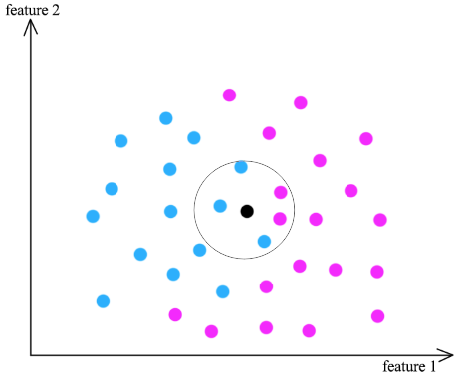
- Find k training data \(x_j\) that are similar to \(x_i\) (the black dot)
- Classification using the result from \(x_j \rightarrow y_j\) (2 pink dots, 3 blue dots)
- No training phase
- Predictions are expensive O(nd)
- We can use different method to measure similarity
- L2 distance
- L1 distance
- Jaccard similarity: \(\frac{count(x_i, x_j)}{count(x_i \text{ or } x_j)}\)
- Cosine similarity
- Distance after dimensionality reduction
- Curse of dimension - High dimensional space need more training data
- Features need to be in similar scale
- Can argument data by translate/rotate/transform images
K-means clustering
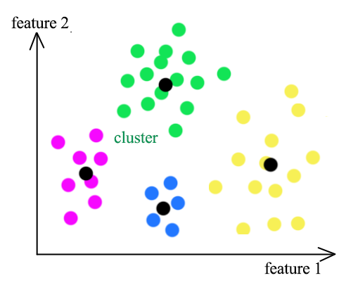
K-means clustering groups datapoints into K clusters. Datapoints are assigned to a cluster with the shortest distance between the datapoint and the centroid of a cluster. (the black dots)
- Pick K random points as centroids
- Form clusters by grouping points to their nearest centroid
- Distance is calculated as the L2 norm
- For points in the same cluster, compute the mean as the new centroid
- Re-cluster all datapoints based on the new centroid location
- Repeat the process in computing the new centroids and re-clustering
- Finish when no points switch to another cluster
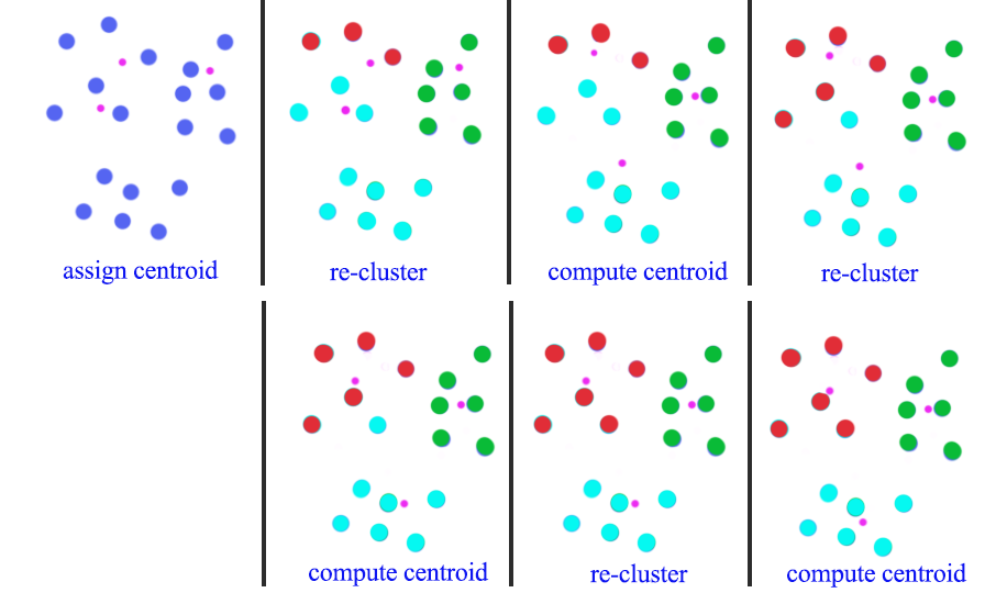
In this diagram, we start with 3 randoms centroids (pink dots). First, we re-cluster all datapoints according to the centroids of the clusters. Then we recompute the new position of the centroids using mean. After 3 iterations of re-clustering and re-calculate, we form 3 clusters.
We can repeat the process many times with different initial random centroids. Then we use the cost function below to select the model with the lowest cost:
\[J = \sum^N_{i=1} \sum^d_{j=1} (x^i_j - c^i_j )^2\]The choices of K can sometimes dictated by the business. For example, a football team only want to partition the stadium into 10 price zones. Therefore, \(k=10\). On the other hand, we can keep increase the value of K until the cost function above does not show a good return in further dividing the datapoints.
Vector quantization
In image vector quantization, we use K-means clustering to map a RGB pixel into one of the cluster’s mean (centroids). For example, we can allocate 8 bits to identify a cluster. Therefore we have \(2^8=256\) clusters. We map a 24 bits RGB pixel into one of the cluster.
\[(234, 255, 34) \rightarrow cluster_{113} \rightarrow 113\]To decode the value of 113, we use the RGB values of the centroid of cluster 113.
\[113 \rightarrow \text{RGB value for } centroid_{113} \rightarrow (220, 248, 30)\]K-median clustering
K-median clustering computes the centroid using the medium. For each dimension, we compute its medium separately from other dimension.
\[c_{i_j} = median_j (x^1_j, x^2_j, \cdots)\]which \(c_{i}\) is the centroid of the cluster \(i\). \(c_{i_j}\) is the \(jth\) dimension of the centroid.
For the cluster assignment, instead of using L2-norm to measure distance, we assign datapoints to the closest cluster with distance measured by the L1 norm.
\[dist^i = \sum^d_{j=1} \vert x^i_j - c_{i_j} \vert\]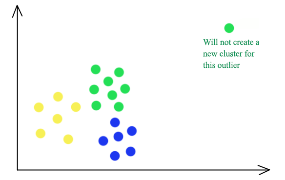
K-median clustering is less vulnerable to outliners. The green outliner on the top right will be grouped into the green cluster in a 3-median cluster instead of having itself as a separate cluster in K-means.
Corresponding cost function:
\[J = \sum^N_{i=1} \sum^d_{j=1} \vert x^i_j - c^i_j \vert\]K-means++ clustering
In K-means clustering, instead of initializing K means (centroids) randomly at the beginning, we random select one mean at a time. We randomly select our first mean. For the next mean, we still select it randomly but with higher preference on datapoints further away from the first mean. For the third mean, we repeat the step with the assigned weight proportional to its distance from the first and the second mean. The selection process continues until we have K means.
- Randomly select a point as the first-mean \(w^1\)
- For all datapoints \(x^i\), compute the distance from all the existing centroids
- Find the distance of each point from its closest centroid
- We pick \(x^i\) randomly as the next centroids with probability proportional to \(dist^i\)
- Repeating the process until we have k-means
Density based clustering (DBSCAN)
As shown below, a distance based cluster like K-means will have problem to cluster concave shape cluster:
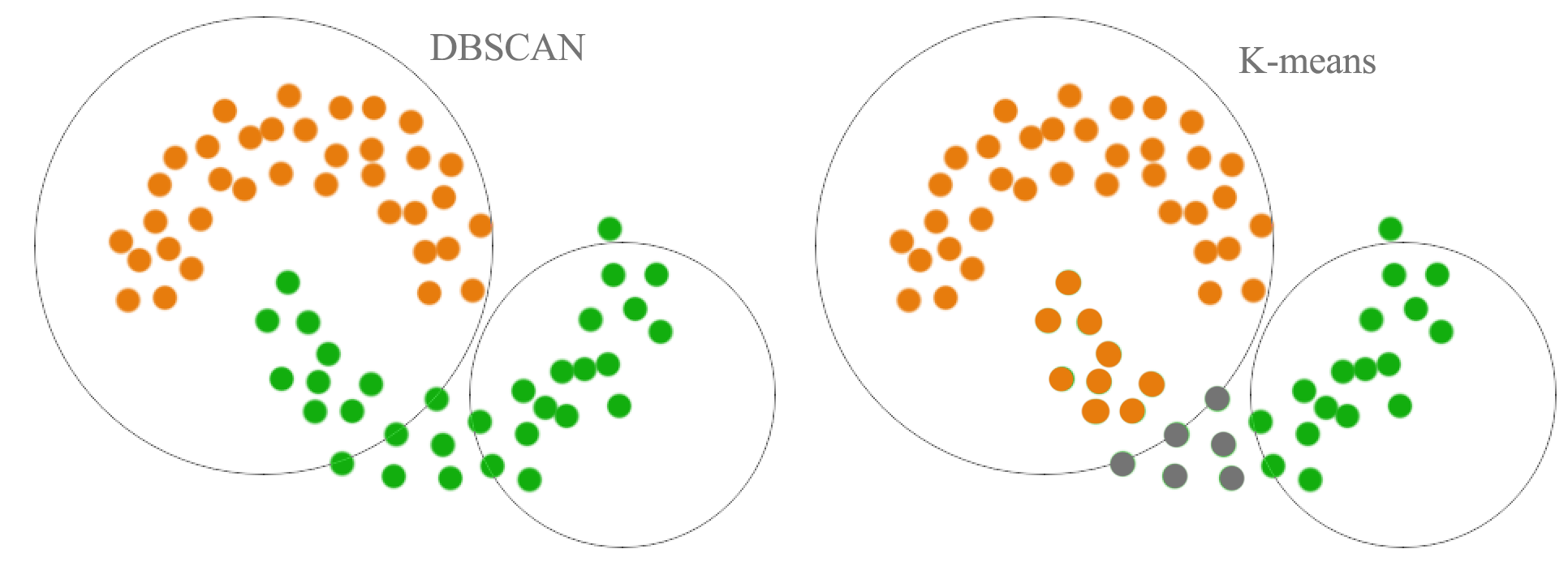
Density based clustering connects neighboring high density points together to form a cluster.
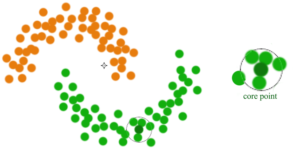
A datapoint is a core point if within radius \(r\), there are \(m\) reachable points. A cluster is form by connecting core points (the darker green) that are reachable from the others.
The green cluster is formed by
- located all the core points (dark green)
- Join all the core points that are within \(r\)
- Join all points that are within \(r\) from all those core points (shown as light green)
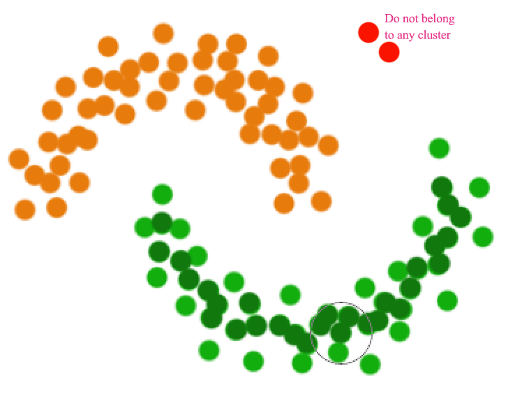
- The green cluster contains both the dark and light green dots
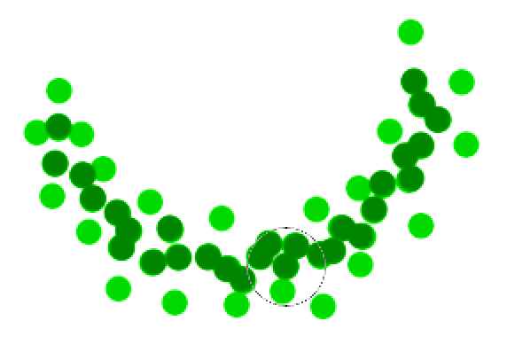
Unlike other clustering, a datapoint may not belong to any cluster.
If we have a lot of datapoints, compute the distances for one datapoints to others are expensive. Instead, datapoints are partitioned into regions. We only connect points that are in the same or adjacent grid regions.
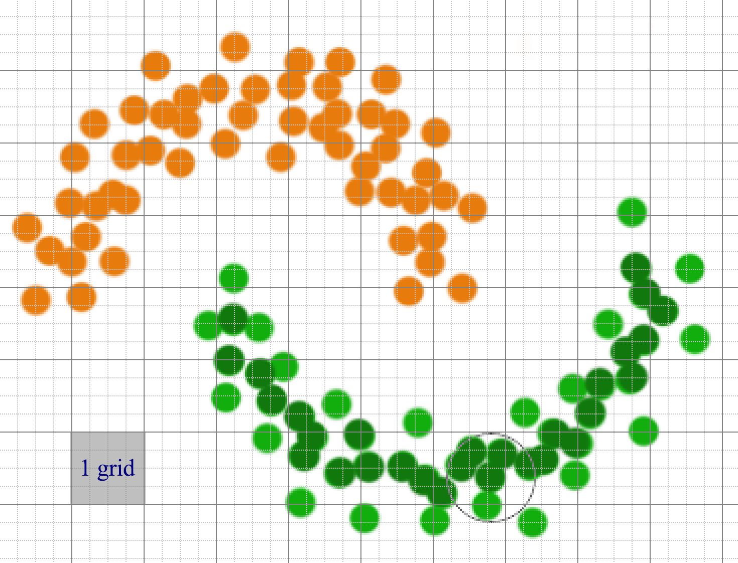
Datapoints can be sparsely distributed. We can use a hash, rather than an array, to store the datapoints that belong to a grid. For feature space with many dimensional, the number of adjacent grid can still be very large though.
Ensemble Clustering (UBClustering)
We can run K-means many times with different initialization to produce many models. Ensemble Clustering usea those models to predict whether 2 datapoints should belong to the same cluster.
- Run K-means M times with different initialization to produce M models
- For datapoints \(x_i\) and \(x_j\), if a simple majority of M models agrees they belongs to the same cluster, make sure they are cluster together.
- If both are already assigned to clusters, merge both clusters.
- If none are assigned, form a new cluster.
- If only one is assigned, assign the other one into the same cluster.
Density-Based Hierarchical Clustering
In Density based clustering (DBSCAN), radius \(r\) acts as a threshold to connect datapoints. The choice of \(r\) can be tricky. When we pick a smaller \(r\), we can detect small scale clusters while a large scale can detect larger clusters.
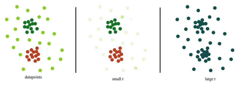
Hierarchical clustering use different size of \(r\) to build a hierarchy of clusters:
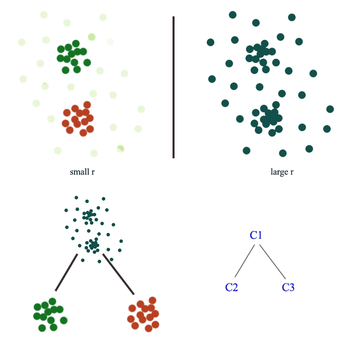
Here is another example:
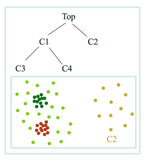
Hierarchical clustering
We can build a hierarchical cluster from bottom-up or bottom down.
Agglomerative clustering (Bottom-Up)
- Starts with each datapoint as its own cluster
- Merge the two closest clusters
- Average-link: Merge 2 clusters with smallest average distance between datapoints after merging
- Single-link: Minimum distance between datapoints
- Complete-link: Maximum distance between datapoints
- Ward’s method: Minimize variance
- Stop when only one cluster left
- More common than bottom-down
Hierarchical K-means (Top-down)
Bottom-down clustering consider all datapoints as one single cluster.
- Use K-means to break a cluster into k clusters
- Continue running k-means for each children cluster
*Until it reaches the total number of clusters that we want or
- The average distance, the radius, the variance, the density or the max distance reaches a threshold
Bisecting K-means
In every iteration, bisecting K-means pick a cluster to split it 2 ways to lower the cost the most.
- Loop until reaching the desired number of clusters or certain threshold has reached
- For every cluster
- Compute the total cost if the cluster is splited into 2 using the K-means clustering
- Pick the cluster that lower the cost the most and commit the split
- For every cluster
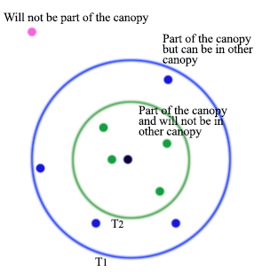
Canopy clustering
Canopy clustering is often used as an initial step to partition datapoints into clusters before moving to a more expensive clustering techniques like K-means clustering.
Canopy clustering using two thresholds
- \(T_1\): the loose distance
- \(T_2\): the tight distance \(T_2<T_1\)
- Start with the set of datapoints to be clustered
- Remove a point from the set as the center of a new canopy
- For each point left in the set, assign it to the new canopy if the distance \(\lt T_1\)
- If the distance of is additionally \(\lt T_2\), remove it from the set
- Repeat from step 2 until there are no more data points in the set
- These relatively cheaply clustered canopies can be sub-clustered using a more expensive algorithm
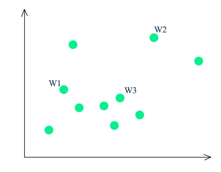
Self-organizing maps (SOM)
Self-organizing maps match feature vectors into one of the node in a lattice. SOM creates a map which neighbors are close to each other. For example, a RGB pixel value is mapped to one of the color node of a color palet created by SOM.

- Each node’s weights \(W_{j}\) are initialized between 0 and 1
- Random select a training dataset \(x_t\)
- Find the node closet to \(x_t\) measured by the L2-norm distance
- The winning node is known as the Best Matching Unit \(u\). (BMU).
- Neighboring nodes \(v\) are adjusted to look closer to \(u\).
- Each \(v\)’s weights are adjusted based on the following equations.
- The closer to the BMU, the more its weights get adjusted.
- The changes also decay with time.
- This adjustment is named \(\theta(u, v, t)\) below.
- \(lr(t)\) is the learning rate like the gradient descent decay with time.
- Repeat the iterations until the solution converge