“Machine learning - Gaussian Process”
Gaussian distribution (Quick review)
We define a function \(y = g(x)\) to map input \(x\) to \(y\). In statistic, we use a stochastic model to define a probability distribution for such relationship. For example, a 3.8 GPA student can earn an average of $60K salary with a variance (\(\sigma^2\)) of $10K.
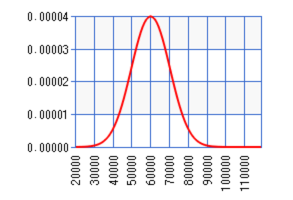
Probability density function (PDF)
In the following diagram, \(p(X=x)\) follows a gaussian distribution:
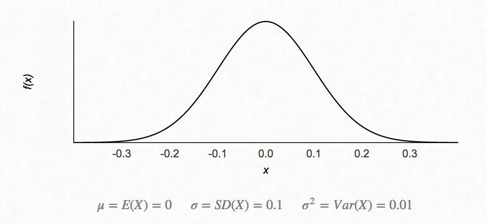
In a Gaussian distribution, 68% of data is within 1 \(\sigma\) from the \(\mu\) and 95% of data is within 2 \(\sigma\).
We can sample data based on the probability distribution. The notation to sample data from a distribution \(\mathcal{N}\) is:
\[x \sim \mathcal{N}{\left( \mu , \sigma^2 \right)}\]In many real world examples, data follows a gaussian distribution.
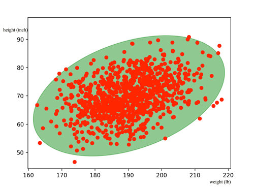
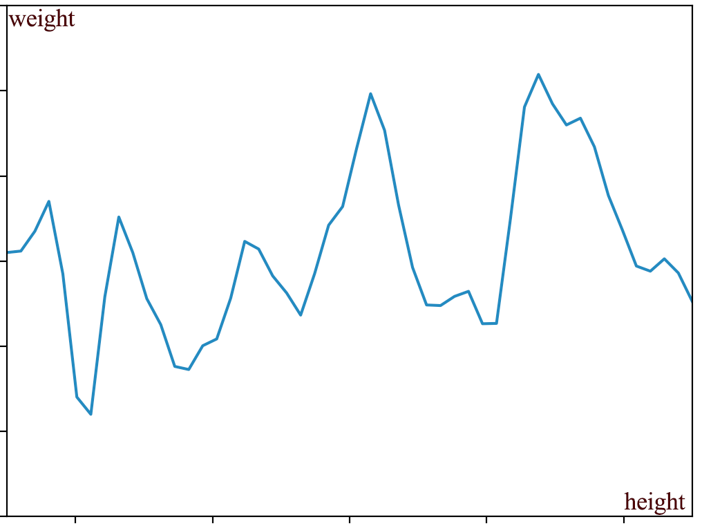
Here, let’s model the relationship between the body height and the body weight for San Francisco residents. We collect the information from 1000 adult residents and plot the data below with each red dot represents 1 person:
The corresponding PDF in 3D:
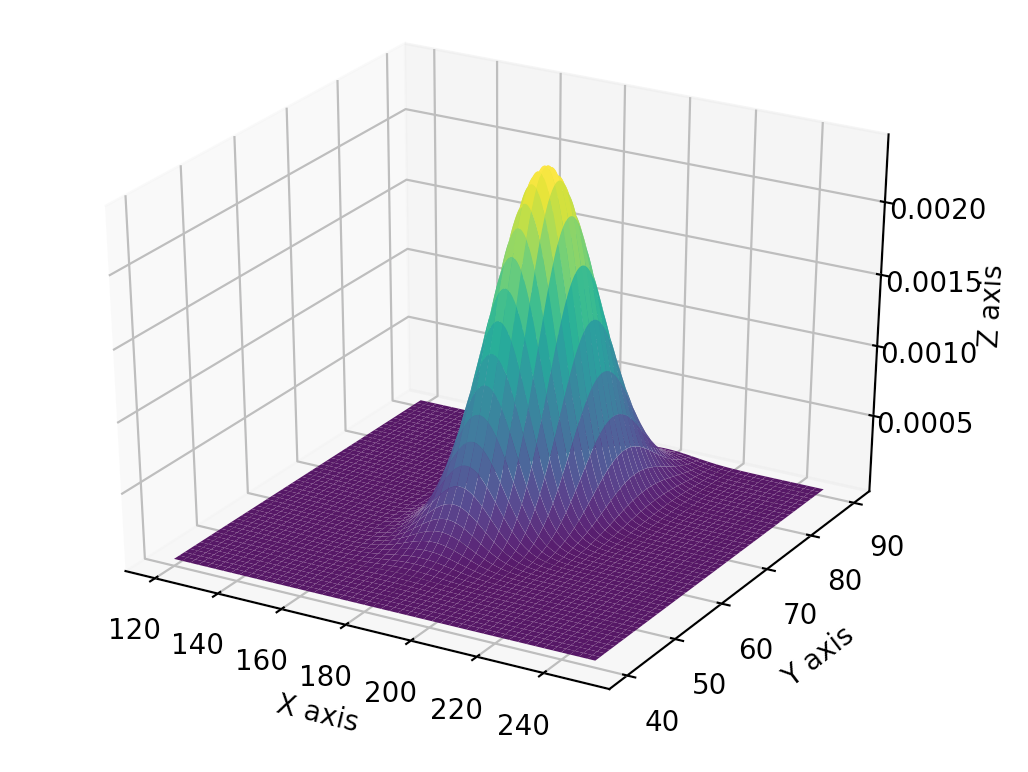
Let us generalize the model first with a multivariate gaussian distribution. i.e. PDF depends on multiple variables.
For a multivariate vector:
\[x = \begin{pmatrix} x_1 \\ \vdots \\ x_p \end{pmatrix}\]The PDF of a multivariate Gaussian distribution is defined as:
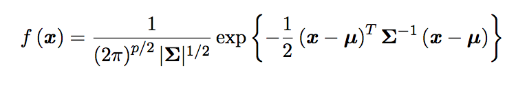
with covariance matrix \(\Sigma\):
\[\Sigma = \begin{pmatrix} E[(x_{1} - \mu_{1})(x_{1} - \mu_{1})] & E[(x_{1} - \mu_{1})(x_{2} - \mu_{2})] & \dots & E[(x_{1} - \mu_{1})(x_{p} - \mu_{p})] \\ E[(x_{2} - \mu_{2})(x_{1} - \mu_{1})] & E[(x_{2} - \mu_{2})(x_{2} - \mu_{2})] & \dots & E[(x_{2} - \mu_{2})(x_{p} - \mu_{p})] \\ \vdots & \vdots & \ddots & \vdots \\ E[(x_{p} - \mu_{p})(x_{1} - \mu_{1})] & E[(x_{p} - \mu_{p})(x_{2} - \mu_{2})] & \dots & E[(x_{n} - \mu_{p})(x_{p} - \mu_{p})] \end{pmatrix}\]Let’s go back to our weight and height example to illustrate it.
\[x = \begin{pmatrix} weight \\ height \end{pmatrix}\]From our training data, we calculate \(\mu_{weight} = 190, \mu_{height} = 70\):
\[\mu = \begin{pmatrix} 190 \\ 70 \end{pmatrix}\]What is the covariance matrix \(\Sigma\) for? Each element in the covariance matrix measures how one variable is related to another. For example, \(E_{21}\) measures how \(\text{height } (x_2)\) is related with \(\text{weight} (x_1)\). If weight increases with height, we expect \(E_{21}\) to be positive.
\[E_{21} = E[(x_{2} - \mu_{2})(x_{1} - \mu_{1})]\]Let’s get into the detail on computing \(E_{21}\) above. To simplify, we consider that we got only 2 data points (150 lb, 66 inches) and (200 lb, 72 inches).
\[E_{21} = E[(x_{2} - \mu_{2})(x_{1} - \mu_{1})] = E[(x_{height} - 70)(x_{weight} - 190)]\] \[E_{21} = E[(x_{height} - 70)(x_{weight} - 190)] = \frac{1}{2} \left( ( 66 - 70) \times (150 - 190) + ( 72 - 70) \times (200 - 190) \right)\]After computing all 1000 data, here is the value of \(\Sigma\):
\[\Sigma = \begin{pmatrix} 100 & 25 \\ 25 & 50 \\ \end{pmatrix}\] \[x \sim \mathcal{N}{\left( \begin{pmatrix} 190 \\ 70 \end{pmatrix} , \begin{pmatrix} 100 & 25 \\ 25 & 50 \\ \end{pmatrix} \right)}\]Positive element values in \(\Sigma\) means 2 variables are positively related. With no surprise, \(E_{21}\) is positive because weight increases with height. If two variables are independent of each other, the value should be 0 like:
\[\Sigma = \begin{pmatrix} 100 & 0 \\ 0 & 50 \\ \end{pmatrix}\]Calculate the probability of \(x < value\)
To calculate the probability of \(X_1 \le z\) given \(X_2 = x\) :
\[P(X_1 \le z\,|\, X_2 = x) = \Phi\left(\frac{z - \rho x}{\sqrt{1-\rho^2}}\right)\]which \(\Phi\) is the accumulative probability distribution:
\[\Phi(a) = \int_{-\infty}^{a} \frac{e^{-(x - \mu)^{2}/(2\sigma^{2}) }} {\sigma\sqrt{2\pi}} dx\]and we rewrote the covariance variable \(\Sigma\) into the following form:
\[\Sigma = \begin{pmatrix} \sigma^2_1 & \rho \sigma_1 \sigma_2 \\ \rho \sigma_1 \sigma_2 & \sigma^2_2 \\ \end{pmatrix}\]Coding
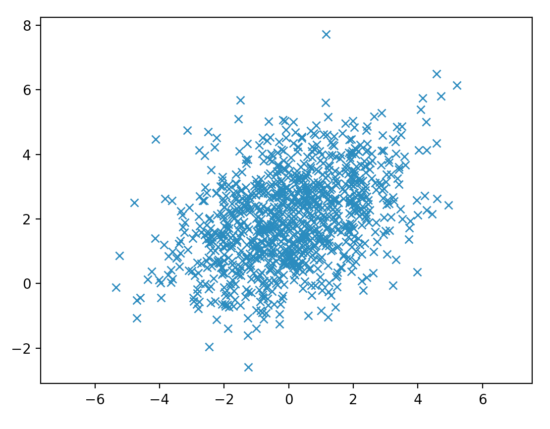
Here we sample data from a 2-variable gaussian distribution. From the covariance matrix, we can tell x is positively related with y as \(\Sigma_{21} \text{ and } \Sigma_{12}\) is positive.
mean = [0, 2]
cov = [[1, 2], [3, 1]]

x, y = np.random.multivariate_normal(mean, cov, 5000).T
plt.plot(x, y, 'x')
plt.axis('equal')
plt.show()
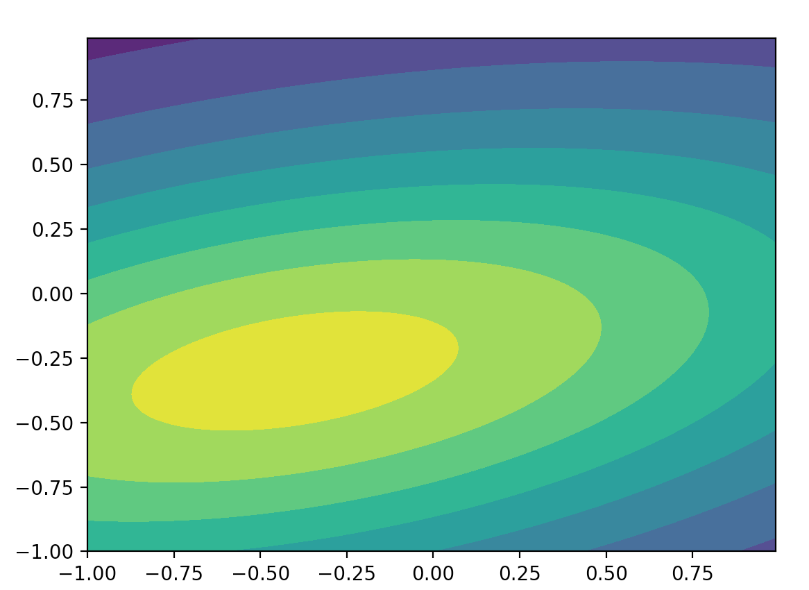
Here, we plot the probability distribution for (y, x).
from scipy.stats import multivariate_normal

x, y = np.mgrid[-1:1:.01, -1:1:.01]  # x (200, 200) y (200, 200)
pos = np.empty(x.shape + (2,))
pos[:, :, 0] = x; pos[:, :, 1] = y   # pos (200, 200, 2)

mean = [-0.4, -0.3]
cov = [[2.1, 0.2], [0.4, 0.5]]
rv = multivariate_normal(mean, cov)
p = rv.pdf(pos)                      # (200, 200)
plt.contourf(x, y, p)
plt.show()
Multivariate Gaussian Theorem
Given a Gaussian Distribution for
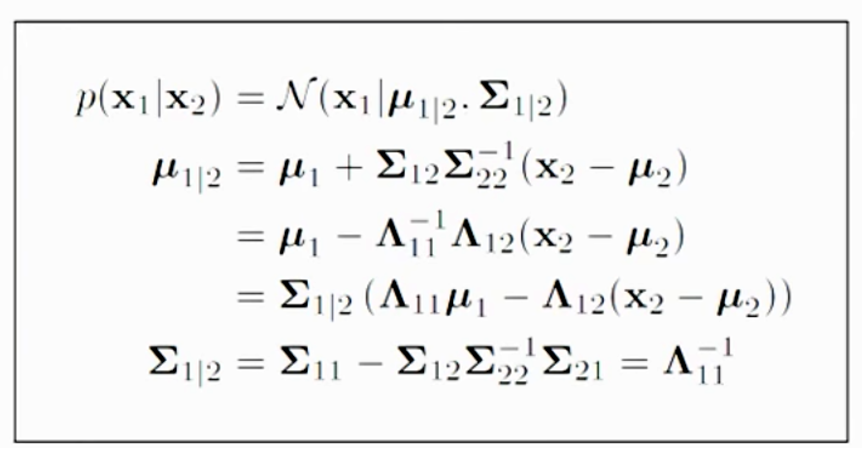
\[x = \begin{pmatrix} x_1\\ x_2 \end{pmatrix} \sim \mathcal{N}{\left( \mu , \Sigma^2 \right)}\]The posterior conditional for \(p(x_1 \vert x_2)\) is given below. This formular is particular important for the Gaussian process in the later section. For example, if we have samples of 1000 graduates with their GPAs and their salaries, we can use this theorem to predict salary given a GPA \(P(salary \vert GPA)\) by creating a Gaussian distribution model with our 1000 training datapoints.
Proof of this theorem can be found here. We will not go into details on the proof. But with the assumption that \(x\) is Gaussian distributed. The co-relation of \(x_1\) and \(x_2\) is defined by \(\mu\) and \(\Sigma\). So given the value of \(x_2\), we can compute the probability distribution of \(x_1\): \(p(x_1 \vert x_2)\)
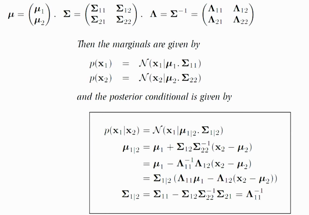
Source: Nando de Freitas UBC Machine learning class.
For example, we know that height of SF residents is gaussian distributed. In the next section, we will apply GP to make a prediction of weight given a height.
Gaussian Process (GP)
The intuition of the Gaussian Process GP is simple. If 2 points have similar input, their output should be similar. With 2 datapoints, if one is closer to a known training datapoint, its prediction is more certain than the other one.
If a student with a GPA 3.5 earns $70K a year, another student with a GPA 3.45 should earn something very similar. In GP, we use our training dataset to build a Gaussian distribution to make prediction. For each prediction, we output a mean and a \(\sigma\). For example, with GP, we can predict a 3.3 GPA student can earn \(\mu = $65K\) with \(\sigma= $5K\) while a 2.5 GPA student can earn \(\mu = $50K\) and \(\sigma= $15K\). \(\sigma\) measures the un-certainty of our prediction. Because a 3.3 GPA is closer to our 3.5 GPA training data, we are more confident about the salary prediction for a 3.3 GPA student than a 2.5 GPA student.
In GP, instead of computing \(\Sigma\), we compute \(K\) trying to measure the similarity between datapoint \(x^i\) and \(x^j\).
| K | \(x^1\) | \(x^2\) | … | \(x^n\) |
| \(x^1\) | 1 | \(k(x^1, x^2)\) | \(k(x^1, x^n)\) | |
| \(x^2\) | \(k(2^1, x^1)\) | 1 | \(k(x^2, x^n)\) | |
| … | ||||
| \(x^n\) | \(k(x^n, x^1)\) | \(k(x^n, x^2)\) | 1 |
which kernel \(k\) is a function measuring the similarity of the 2 datapoints (1 means the same). There are many possible kernel functions, we will use an exponential square distance for our kernel.
\[K_{i,j} = k(x^i, x^j) = e^{-\frac{1}{2}(x^i - x^j)^2}\]Note: In previous section \(x_1\) means the weight of a datapoint. Here \(x^1\) means datapoint 1. \(X^x_1\) means the weight of datapoint 3.
With all the training data, we can create a Gaussian model:
\[\begin{pmatrix} f \end{pmatrix} \sim \mathcal{N}{\left( \mu , K \right)}\]Let’s demonstrate it again with 2 training datapoints (150 lb, 66 inches) and (200lb, 72 inches). Here we are building a Gaussian model for our training data.
\[\begin{pmatrix} 150 \\ 200 \end{pmatrix} \sim \mathcal{N}{\left( 175 , \begin{pmatrix} K_{11} & K_{12}\\ K_{21} & K_{22} \end{pmatrix} \right)}\]with 175 as the mean of the weight and \(K_{i,j} = k(x^i, x^j)\) measures the similarity of the height of the datapoints \(x^i, x^j\). The notation above just mean we can sample a vector \(f\) on weight
\[f = \begin{pmatrix} 150 \\ 200 \end{pmatrix}\]from \(\mathcal{N}\) which is model by the datapoint (150, 66) and (200, 72).
Now let’s say we want to predict \(f^1, f^2\) for input \(x^{1}_*, x^{2}_*\). The model change to:
\[\begin{pmatrix} 150 \\ 200 \\ f^1 \\ f^2 \\ \end{pmatrix} \sim \mathcal{N}{\left( 175 , \begin{pmatrix} K_{11} & K_{12} & K_{13} & K_{14} \\ K_{21} & K_{22} & K_{23} & K_{24} \\ K_{31} & K_{32} & K_{33} & K_{34} \\ K_{41} & K_{42} & K_{43} & K_{44} \\ \end{pmatrix} \right)}\]Let’s understand what does it mean again. For example, we have a vector contain 4 persons height
\[x = (66, 72, 67, 68)\]We can use \(\mathcal{N}\) to sample the possible weight for these people:
\[(150, 200, f^1, f^2)\]We know the first 2 values from the training data and we try to compute the distribution for \(f^1 \text{and } f^2\). (what is their \(\mu\) and \(\sigma\).) Now, instead of predicting just 2 values, we can have input over a range of values
\[x = (66, 72, 0, 0.01, 0.02, ..., 65.99, 66, 66.01, ... )\]and use \(\mathcal{N}\) to sample vector:
\[(150, 200, f^1, f^2, f^3, ...)\]For example, our first output sample from \(\mathcal{N}\) is
\[(150, 200, 0, 0.02, 0.05, ..., 149.2, 150, 148.4, ...)\]We can plot the output against input. The line below is just a regular non-scholastic function. i.e. \(weight = g(height) \text{ or } y = g(x)\).
In this section, we use the notation \(g(x)\) as a non-scholastic function while \(f(x)\) as a scholastic function.
To generate training data much easier, we are switching to a new model \(y = \sin(x)\). We use the equation to generate 2 training datapoints (2 blue dots below) to build a Gaussian model. We then sample \(\mathcal{N}\) three times shown as the three solid lines below.
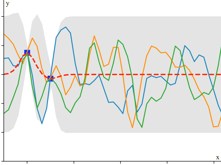
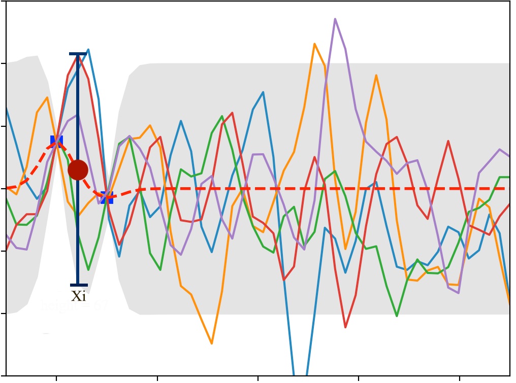
We see that the 2 training data forces \(\mathcal{N}\) to have all lines interest at the blue dots. If we keep sampling, we will start visually recognize the mean and the range of \(y_i\) for each \(x_i\). For example, the red dot and the blue line below estimates the mean and the variance of \(y_i\) for \(x_i=-3.8)\). Since \(x_i\) is between 2 training points, the estimation has a relatively high un-certainty (indicated by \(\sigma\)).
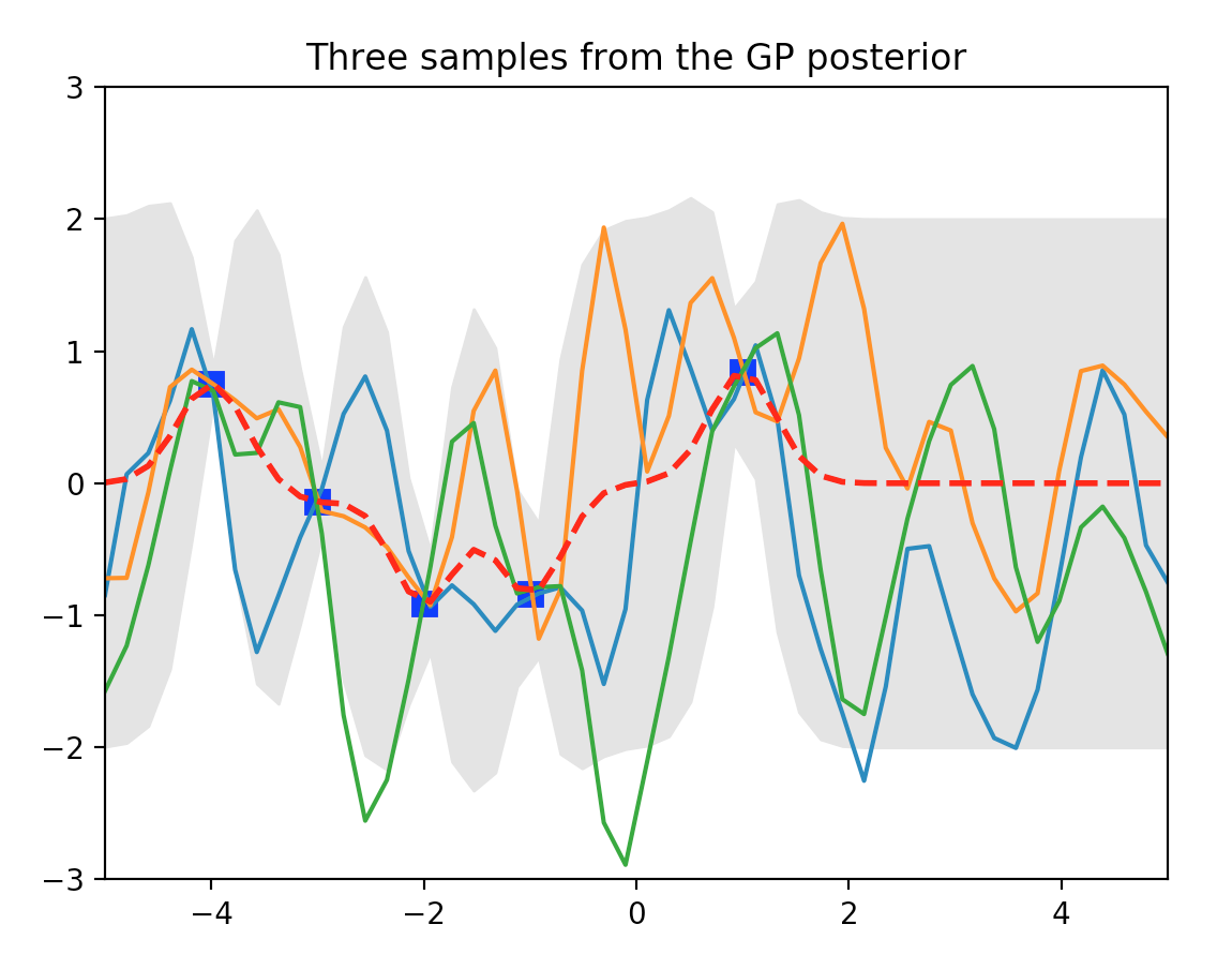
In the plot below, we have 5 training data and we sample 30 lines from \(\mathcal{N}\). The red dotted line indicates the mean output value \(\mu_i\) for \(y_i\) and the gray area are within 2 \(\sigma_i\) from \(\mu_i\).
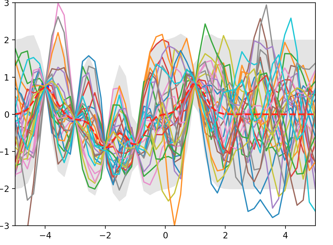
As mentioned before, each line acts like a function to map input to output: \(y = g(x)\). We start with many possible functions \(g\) but the training dataset reduce or increase the likelihood of some functions. Technically, \(\mathcal{N}\) model the possibility distribution of the functions \(g\) given the training dataset. (the probability distribution of the lines drawn above.)
GP is charactered as building a Gaussian model to discribe the distribution of functions.
We are not going to solve the problem by sampling. Instead we will solve it analytically.
Back to
\[\begin{pmatrix} 150 \\ 200 \\ f^1 \\ f^2 \\ \end{pmatrix} \sim \mathcal{N}{\left( 175 , \begin{pmatrix} K_{11} & K_{12} & K_{13} & K_{14} \\ K_{21} & K_{22} & K_{23} & K_{24} \\ K_{31} & K_{32} & K_{33} & K_{34} \\ K_{41} & K_{42} & K_{43} & K_{44} \\ \end{pmatrix} \right)}\]We can generalize the expression as follow which \(f\) is the label (weights) of the training set and \(f_{*}\) is the weights that we want to predict for \(x_*\). Now we need to solve \(p(f_* \vert f)\) with the Gaussian model.
\[\begin{pmatrix} f \\ f_{*} \end{pmatrix} \sim \mathcal{N}{\left( \begin{pmatrix} \mu \\ \mu_{*} \end{pmatrix} , \begin{pmatrix} K & K_{s}\\ K_{s}^T & K_{ss}\\ \end{pmatrix} \right)}\] \[\text{which } f = \begin{pmatrix} 150 \\ 200 \end{pmatrix} \text{ and } f_* = \begin{pmatrix} f^1 \\ f^2 \end{pmatrix}\]Recall from the previous section on Multivariate Gaussian Theorem, if we have a model
\[\begin{pmatrix} x_1 \\ x_2 \end{pmatrix} \sim \mathcal{N}{\left( \begin{pmatrix} \mu_1 \\ \mu_2 \end{pmatrix} , \begin{pmatrix} \Sigma_{11} & \Sigma_{12} \\ \Sigma_{21} & \Sigma_{22} \\ \end{pmatrix} \right)}\]We can solve \(p(x_1 \vert x_2)\) by:
Now, we apply the equations to solve
\[p(f_{*} \vert f)\]For the training dataset, let output labels \(f\) has the gaussian distribution:
\[\begin{split} f & \sim \mathcal{N}{\left(\mu, \sigma^2\right)} \\ & \sim \mu + \sigma(\mathcal{N}{\left(0, 1\right)}) \\ \end{split}\]And let the Gaussian distribution for \(f_{*}\) be:
\[\begin{split} f_{*} & \sim \mathcal{N}{\left(\overline{\mu}_{*}, \overline{\Sigma}_{*}\right) } \\ & \sim \overline{\mu}_{*} + L\mathcal{N}{(0, I)} \end{split}\]which L is defined as
\[LL^T = \overline{\Sigma}_{*}\]and from the Multivariate Gaussian Theorem:
\[\begin{split} p(f_*\vert x_*, x, f) & = \mathcal N( \mu_{*} + K_{ s}^T K^{-1}( f - \mu ), K_{ss} - K_{s}^T K^{-1} K_{s}) \\ \overline{\mu}_{*} & = \mu_{*} + K_{ s}^T K^{-1}( f - \mu ) \\ \overline{\Sigma}_{*} & = K_{ss} - K_{s}^T K^{-1} K_{s} \end{split}\]We are applying the equations to model training data from \(y = \sin(x)\). In this example, \(\mu=\mu_{*}=0\) as the mean value of a \(sin\) function is 0. Our equation will therefore simplify to:
\[\begin{split} \overline{\mu}_{*} & = K_{ s}^T K^{-1} f \\ \overline{\Sigma}_{*} & = K_{ss} - K_{s}^T K^{-1} K_{s}\\ K & = L L^T \quad \text{(use Cholesky to decompose K)} \end{split}\]Note, \(K\) may be poorly condition to find the inverse. So we apply Cholesky to decompose K first and then apply linear algebra to solve \(K_{ s}^T K^{-1} f\).
The notation
\[x = A \backslash b\]means using linear algebra to solve x for \(Ax=b\) .
We are going to pre-compute some terms before solving \(K_{ s}^T K^{-1} f\).
\[\begin{split} \text{Let u be } u &= L^{-1} f \\ Lu &= f \\ u &= L \backslash f = L^{-1} f \\ \text{Let v be } v &= L^{-T} u = L^{-T} L^{-1} f \\ L^{T}v &= u \\ v &= L^{T} \backslash u \\ &= L^{T} \backslash (L \backslash f) = L^{-T} L^{-1} f \end{split}\]Apply \(K = LL^{T}\) and the equation above
\[\begin{split} \overline{\mu}_{*} & = K_{ s}^T K^{-1} f \\ & = K_{ s}^T (LL^{T})^{-1} f \\ & = K_{ s}^T L^{-T}L^{-1} f \\ & = K_{ s}^T L^T \backslash ( L \backslash f ) \\ \end{split}\]Now, we we have the equations to compute \(\overline{\mu}_{*}\) and \(\overline{\Sigma}_{*}\).
Coding
First we are going to prepare our training data and label it with a \(\sin\) function. The training data contains 5 datapoints. \((x_i=-4, -3, -2, -1 \text{ and} 1)\).
Xtrain = np.array([-4, -3, -2, -1, 1]).reshape(5,1)
ytrain = np.sin(Xtrain)      # Our output labels.
Testing data: We create 50 new datapoint linear distributed between -5 and 5 to be predicted by the Gaussian process.
# 50 Test data
n = 50
Xtest = np.linspace(-5, 5, n).reshape(-1,1)
Here we define a kernel measure the similarity of 2 datapoint using an exponential square kernel.
# A kernel function (aka Gaussian) measuring the similarity between a and b. 1 means the same.
def kernel(a, b, param):
    sqdist = np.sum(a**2,1).reshape(-1,1) + np.sum(b**2,1) - 2*np.dot(a, b.T)
    return np.exp(-.5 * (1/param) * sqdist)
To compute the Kernel (\(K, K_s, K_{ss})\)
K = kernel(Xtrain, Xtrain, param)                        # Shape (5, 5)
K_s = kernel(Xtrain, Xtest, param)                       # Shape (5, 50)
K_ss = kernel(Xtest, Xtest, param)                       # Kss Shape (50, 50)
We will use the Cholesky decomposition to decompose \(K = LL^T\).
L = np.linalg.cholesky(K + 0.00005*np.eye(len(Xtrain))) # Shape (5, 5)
Compute the mean output \(\overline{\mu}_*\) for our prediction. As we assumem \(\mu_{*} = \mu = 0\), the equation becomes:
\[\begin{split} \overline{\mu}_{*} & = K_{ s}^T K^{-1} f \\ & = K_{ s}^T L^T \backslash ( L \backslash f ) \end{split}\]L = np.linalg.cholesky(K + 0.00005*np.eye(len(Xtrain))) # Add some nose to make the solution stable
# Shape (5, 5)
# Compute the mean at our test points.
Lk = np.linalg.solve(L, K_s) # Shape (5, 50)
mu = np.dot(Lk.T, np.linalg.solve(L, ytrain)).reshape((n,)) # Shape (50, )
Compute \(\sigma\)
# Compute the standard deviation.
s2 = np.diag(K_ss) - np.sum(Lk**2, axis=0)               # Shape (50, )
stdv = np.sqrt(s2)                                       # Shape (50, )
Sample \(f_*\) so we can plot it.
\[\begin{split} \overline{\Sigma}_{*} & = K_{ss} - K_{s}^T K^{-1} K_{s} \\ \overline{\Sigma}_{*} & = LL^T \\ \end{split}\]Sample it using \(\mu\), and \(L\) as variance:
\[f_* \sim \overline{\mu}_{*} + L\mathcal{N}{(0, I)}\]L = np.linalg.cholesky(K_ss + 1e-6*np.eye(n) - np.dot(Lk.T, Lk)) # Shape (50, 50)
f_post = mu.reshape(-1,1) + np.dot(L, np.random.normal(size=(n,5))) # Shape (50, 3)
We sample 3 possible output shown in orange, blue and green line. The gray area is where within 2 \(\sigma\) of \(\mu\). Blue dot is our training dataset. Here, at blue dot, \(\sigma\) is closer to 0. For points between the training datapoints, \(\sigma\) increases reflect its un-certainty because it is not close to the training dataset points. When we move beyond \(x=1\), we do not have any more training data and result in large \(\sigma\).
Here is another plot of posterior after seeing 5 evidence. The blue dot is where we have training datapoint and the gray area demonstrate the un-certainty (variance) of the prediction.
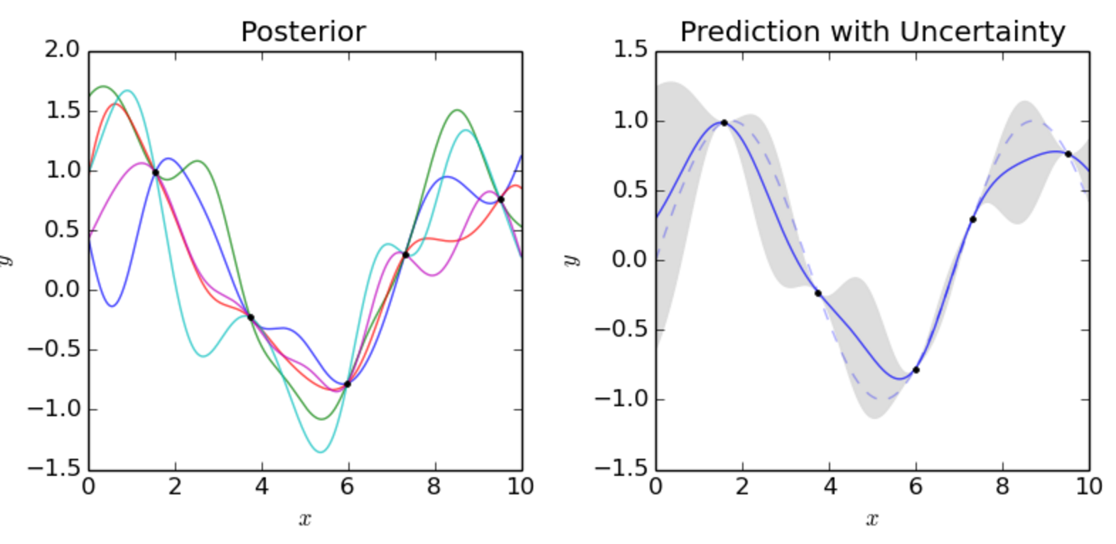
Source Wikipedia.
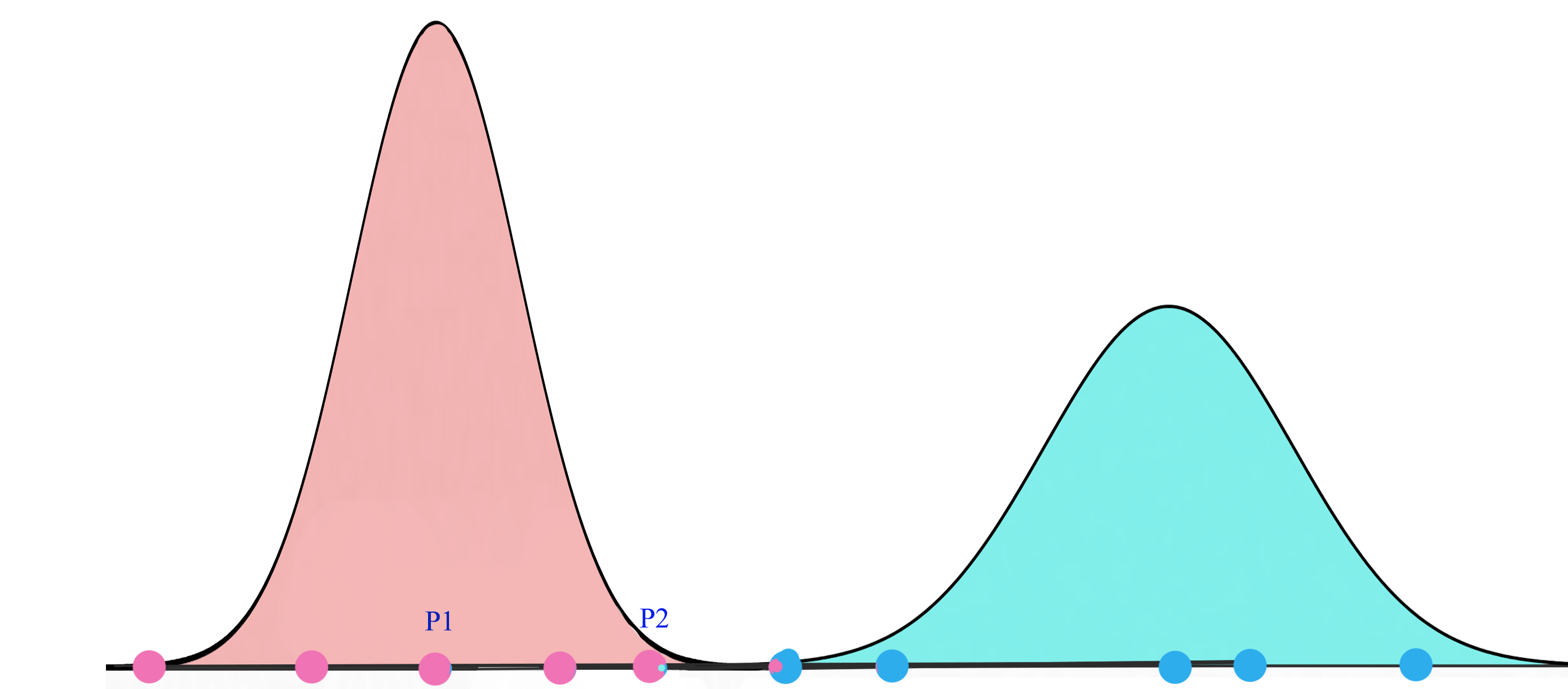
Gaussian mixture model
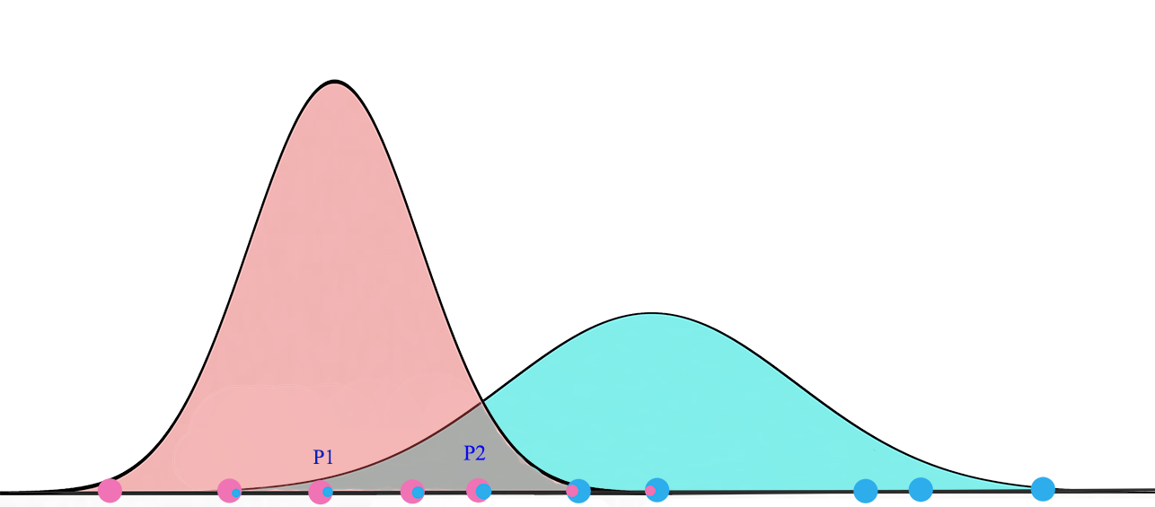
A Gaussian mixture model is a probabilistic model that assumes all the data points are generated from a mixture of Gaussian distributions.
For K=2, we will have 2 Gaussian distributions \(G_1 = (\mu_1, \sigma^2_1)\) and \(G_2 = (\mu_2, \sigma^2_2)\). We start with a random initialization of parameters \(\mu\) and \(\sigma\). Gaussian mixture model tries to fit the training datapoints into \(G_1\) and \(G_2\) and then re-compute their parameters. The datapoints are re-fitted and the parameters are re-calculated again. The iterations continues until the solution converges.
Expectation Maximization (EM)
Details in Expectation Maximization:
- Initialize the \(G1\) and \(G2\)’s parameters \((\mu_1, \sigma^2_1)\) and \((\mu_2, \sigma^2_2)\) with random values. Set \(P(a)=P(b)=0.5\)
- For all the training datapoints \(x_1, x_2, \cdots\), compute the probability that it belongs to \(a\) (\(G_1\)) or \(b\) (\(G_2\)).
- Now, we recalculate the parameters for \(G_1\) and \(G_2\)
- Recalculate the priors
For Gaussian Distribution with multiple variate, the probability distribution function is:
\[P(x_i \vert b) = \frac{1}{\sqrt{(2\pi)^n \vert \Sigma_b \vert}}e^{- \frac{1}{2}(x - \mu_b)^T \Sigma_b^{-1} (x - \mu_b)} \\\]