“Machine learning - Notes”
Bias and variance
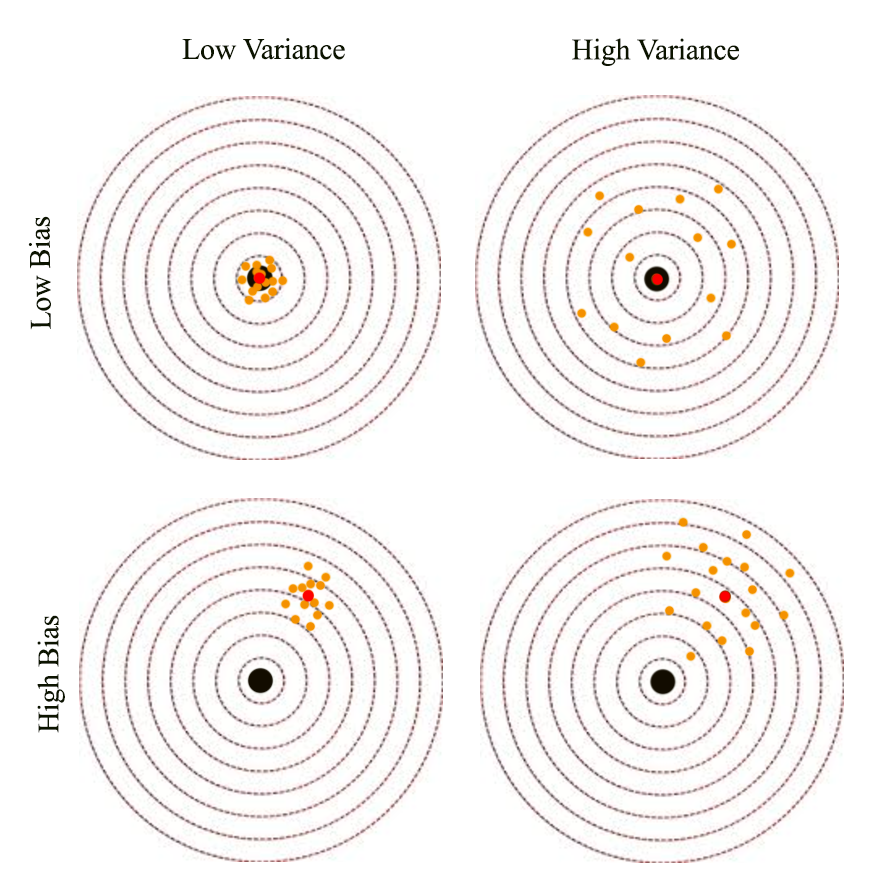
There are two sources of error. The variance is error sensitivity to small changes in the training set. It is often the result of overfitting: powerful model but not enough data. On the other hand, bias happens when the model is not powerful enough to make accurate prediction (underfitting). Usually a high variance but low bias model makes in-consistence prediction when trained with different batches of input. But the average prediction is close to the true value. The orange dots below are predictions make by a deep network. The predictions made by a highly variance model generate predictions widely spread around the true value. A highly variance model make consistence predictions but it is off from the true value.
We define bias and variance as:
\[\begin{split} bias(\hat\theta) & = \mathbb{E}_{p(D\vert \theta_0)} (\hat\theta) - \theta_0 = \overline\theta - \theta_0 \\ \mathbb{V} (\hat\theta) & = \mathbb{E}_{p(D\vert \theta_0)} (\hat\theta - \overline\theta)^2 \\ \end{split}\]Here we proof that the mean square error is actually compose of a bias and a variance.
\[\begin{split} MSE & = \mathbb{E} (\hat\theta - \theta_0)^2 \\ & = \mathbb{E} [2 (\overline\theta^2 - \theta_0 \overline\theta - \overline\theta \hat \theta - \theta_0 \hat\theta) + (\hat\theta - \theta_0)^2] \\ & = \mathbb{E} [\overline\theta^2 - 2 \theta_0 \overline\theta + \overline\theta^2] + \mathbb{E} [\overline\theta^2 - 2 \overline\theta \hat \theta + \overline\theta^2)] \\ & = (\overline\theta - \theta_0)^2 + \mathbb{E} (\hat\theta - \overline\theta)^2 \\ & = bias(\hat\theta)^2 + \mathbb{V} (\hat\theta) \\ \end{split}\]Given:
\[\begin{split} & \mathbb{E} (\overline\theta^2 - \theta_0 \overline\theta - \overline\theta \hat \theta - \theta_0 \hat\theta) \\ & = \overline\theta^2 - \theta_0\overline\theta - \overline\theta^2 - \theta_0\overline\theta \\ & = 0 \\ \end{split}\]Simple model has high bias. Overfitting a high complexity model causes high variance.
Example: Gaussian distribution estimator
Gaussian equation:
\[\mathcal{N}(x;μ, σ^2) = \frac{1}{\sigma\sqrt{2\pi}}e^{-(x - \mu)^{2}/2\sigma^{2} }\]A common estimator for the Gaussian mean parameter:
\[\begin{split} \hat{\mu}_m = \frac{1}{m} \sum^m_1 x_i \\ \end{split}\]Estimate the Bias of the estimator:
\[\begin{split} bias(\hat{\mu}_m ) &= \mathbb{E}[\hat{\mu}_m ] - \mu \\ &= \mathbb{E} [\frac{1}{m} \sum^m_1 x_i ] - \mu \\ &= \frac{1}{m} \mathbb{E} [\sum^m_1 x_i ] - \mu \\ &= \frac{1}{m} m \mathbb{E}[x_i] - \mu \\ &= \mu - \mu \\ &= 0 \\ \end{split}\]Hence, our estimator for the Gaussian mean parameter has zero bias.
Let’s consider the following estimator for the Gaussian variance parameter:
\[\begin{split} \hat{\sigma}^2_m = \frac{1}{m} \sum^m_{i=1} (x_i - \hat{\mu_m})^2 \\ \end{split}\]Estimate the Bias of the estimator:
\[\begin{split} bias(\hat{\sigma}^2_m) = \mathbb{E} [\hat{\sigma}^2_m] - \sigma^2 \end{split}\]Calculate \(\mathbb{E} [\hat{\sigma}^2_m]\) first:
\[\begin{split} \mathbb{E} [\hat{\sigma}^2_m] & = \mathbb{E} [\frac{1}{m}\sum_{i = 1}^N (x_i - \mu_m)^2] = \frac{1}{m} \mathbb{E} [\sum_{i = 1}^m (x_i^2 - 2x_i \mu_m + \mu_m^2)] \\ & = \frac{1}{m} \big( \mathbb{E} [\sum_{i = 1}^m x_i^2] - \mathbb{E} [\sum_{i = 1}^m 2x_i \mu_m] + \mathbb{E} [\sum_{i = 1}^m \mu_m^2)] \big) \\ & = \frac{1}{m} \big( \mathbb{E} [\sum_{i = 1}^m x_i^2] - \mathbb{E} [\sum_{i = 1}^m 2 \mu_m \mu_m] + \mathbb{E} [\sum_{i = 1}^m \mu_m^2)] \big) \\ &= \frac{1}{m} \big( \mathbb{E} [\sum_{i = 1}^m x_i^2] - \mathbb{E} [\sum_{i = 1}^m \mu_m^2)] \big) \\ &= \mathbb{E} [x_m^2] - \mathbb{E} [\mu_m^2)] \\ & = \sigma_{x_m}^2 + \mu_{x_m}^2 - \sigma_{\mu_m}^2 - \mu_{\mu_m}^2 \quad \text{since }\sigma^2 = \mathbb{E} [x^2] - \mu^2 \implies \mathbb{E} [x^2] = \sigma^2 + \mu^2 \\ & = \sigma_{x_m}^2 - \sigma_{\mu_m}^2 \quad \text{since } \mu_{x_m}^2 = \mu_{\mu_m}^2 \\ & = \sigma_{x_m}^2 - Var(\mu_m) \\ & = \sigma_{x_m}^2 - Var( \frac{1}{m} \sum^m_{i=1} x_m) \\ & = \sigma_{x_m}^2 - \frac{1}{m^2} Var(\sum^m_{i=1} x_m) \\ & = \sigma_{x_m}^2 - \frac{1}{m^2} m \sigma_{x_m}^2 \\ & = \frac{m-1}{m} \sigma_{x_m}^2 \neq 0\\ \end{split}\]Hence, this estimator is biased. Intuitively, we sometimes over-estimate and sometimes estimate \(\mu\). By squaring it, we tends to over-estimate all the time and therefore the estimator has biases. The correct estimator for \(\sigma\) is:
\[\begin{split} \hat{\sigma}^2_m = \frac{1}{m-1} \sum^m_{i=1} (x_i - \hat{\mu_m})^2 \\ \end{split}\]Proof:
\[\begin{split} \mathbb{E} [\hat{\sigma}^2_m] & = \mathbb{E} [ \frac{1}{m-1} \sum^m_{i=1} (x_i - \mu_m)^2 ] \\ & = \frac{1}{m-1} \mathbb{E} [ \sum^m_{i=1} (x_i - \mu_m)^2 ] \\ & = \frac{1}{m-1} (m-1) \mathbb{E} [ \sigma^2_{x_m}] \quad \text{reuse the result from the calculations of } \mathbb{E} [\hat{\sigma}^2_m]. \\ & = \sigma^2_{x_m} \\ \end{split}\]L1 regularization
\[\begin{split} J(W) & = \frac{1}{2} \| xw - y \|^2 + \frac{\lambda}{2} \vert w \vert & = MSE + \text{ regularization cost } \end{split}\]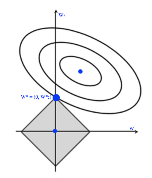
L1 regularization has a tendency to push \(w_i\) to exactly 0. Therefore, L1-regularization increases the sparsity of \(W\).
L2 regularization
\[\begin{split} J(W) & = \frac{1}{2} \| xw - y \|^2 + \frac{\lambda}{2} \| w \|^2 & = MSE + \text{ regularization cost } \end{split}\]\(W^*_a\) is where regularization cost is 0 and \(W^*_b\) is where MSE is minimum. The optimal solution for \(J\) is where the concentric circle meet with the eclipse. This is the same as minimizing mean square error with the L2-norm constraint.
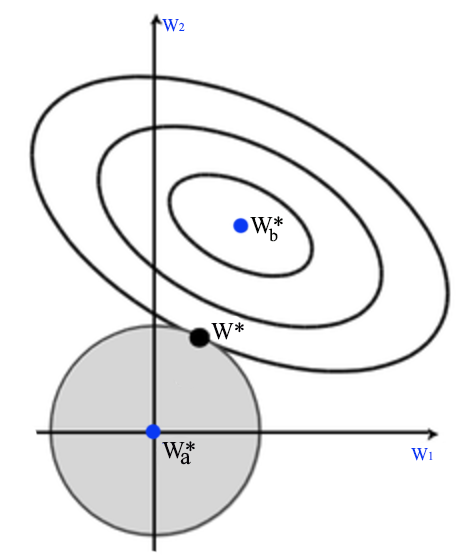
MSE with L2-regularization is also called ridge regression.
L1 vs L2 norm
Even the squared L2-norm may be mathematically simpler and easier to differentiate, the value increases very slowly at the origin. For some machine learning applications, the sparsity of \(W\) is important. In this situration, we may consider L1-norm instead.
Histogram of gradients
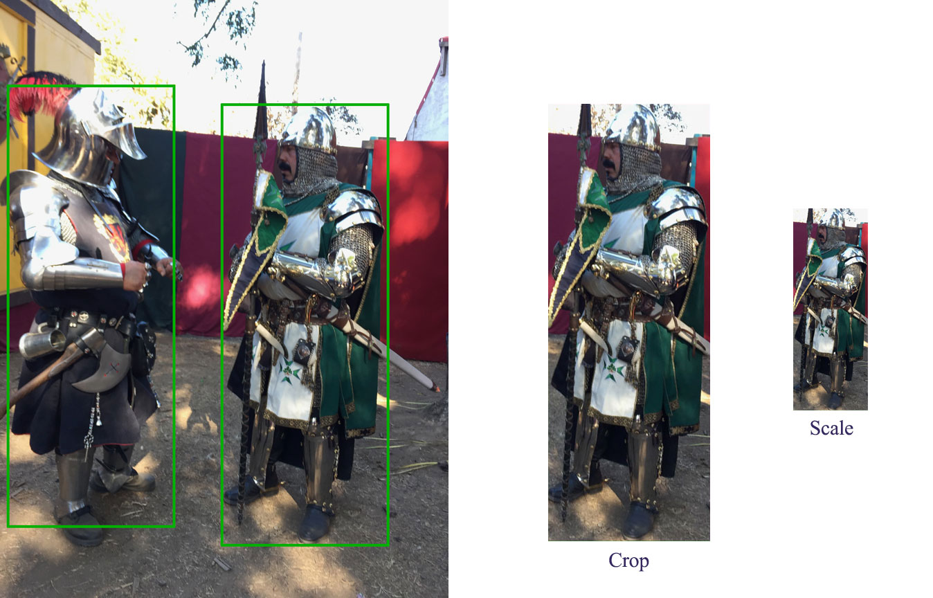
Preprocessing
Crop and scale the image to a fixed size patch.
Calculate gradient
Calculate the gradient at each pixel by subtracting its vertical or horizontal neighbors.
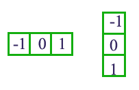
The gradient angle \(\theta\) is from 0 to 360 degree. But we will treat \(\theta\) in the opposite direction to be the same. Therefore, our gradient angle is from 0 to 180 degree. Experiment indicates it performs better in pedestrian detection.
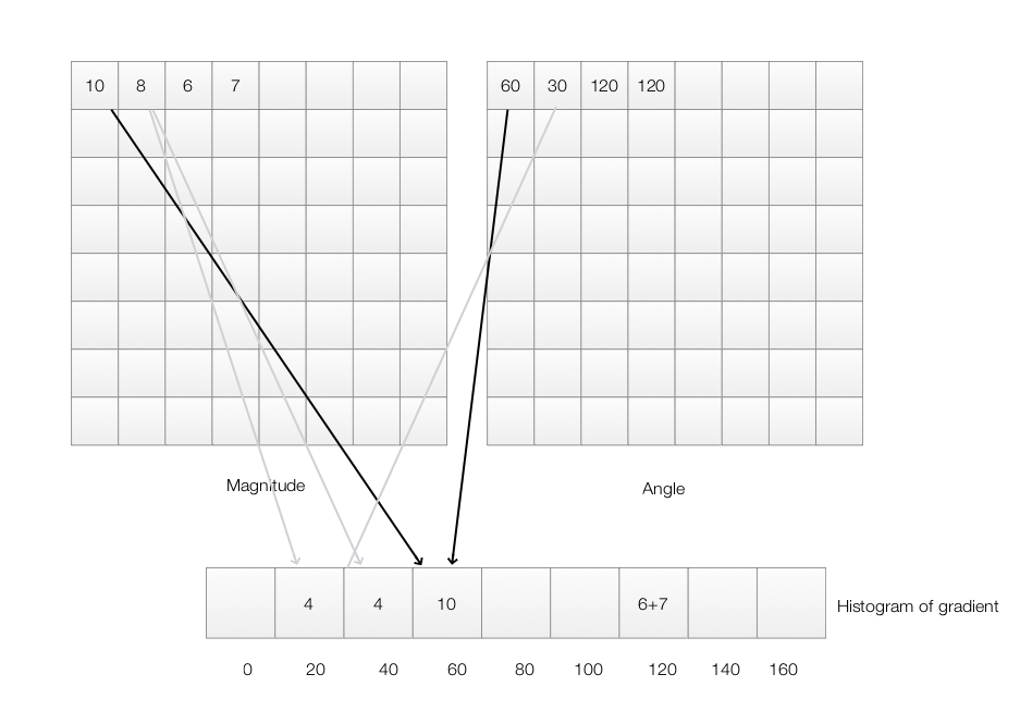
\[\begin{align} \theta_1 &= \vert \arctan \frac{g_y}{g_x} \vert \\ \theta_2 &= \vert \arctan \frac{- g_y}{g_x} \vert = \vert - \arctan \frac{g_y}{g_x} \vert = \vert \arctan \frac{g_y}{g_x} \vert \\ \theta_1 &= \theta_2 \\ \end{align}\]We will compute a histogram for each 8x8 image patch. The histogram has 9 bins starting with \(\theta =0 , 20, 40, 60, 80, 100, 120, 140, 160\). For the first pixel with \(\theta=60, magnitude=10\), we add 10 into the bin \(60\). For the second pixel, we have \(\theta=30, magnitude=8\), this value falls between bin \(20\) and \(30\). We will split it proportionally to the distance from the corresponding bin. In this case, half of the value (\(4\)) goes to bin \(20\) and half goes to bin \(40\). Will goes through every pixels and add values to the corresponding bins. For each 8x8 image patch, we will have an input features with 9 values.
Normalization
Images with different lighting will result in different gradients. We apply normalization so the histogram is not sensitive to lighting.
For each 8x8 patch, we have 9 histogram values, we can normalized each value by the equation below.
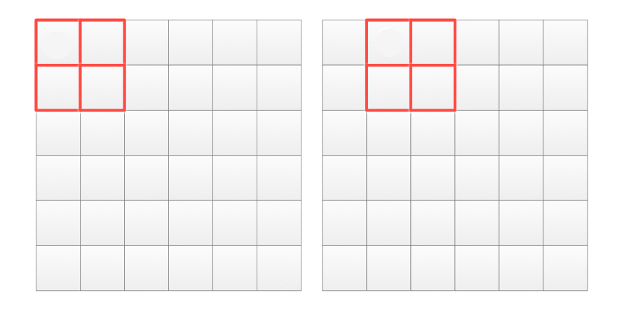
\[h_i = \frac{h_i}{\sqrt{ h_1^2 + h_2^2 + \cdots + h_9^2} }\]It can be shown easily that even we double every \(h_i\), the normalized value remains the same. Hence, we reduce its sensitivity to lighting. We are going to make one more improvement. Instead of normalize every patch, we normalize 4 patches with a sliding window. In the red rectangle below, it compose of 4 patches (16x16 pixels) corresponding to 4x9 histogram values. We are going to generate 4x9 normalized features as:
\[h_i = \frac{h_i}{\sqrt{ h_{11}^2 + \cdots + h_{19}^2 + h_{21}^2 + \cdots + h_{29}^2 + h_{31}^2 + \cdots + h_{39}^2 + h_{41}^2 + \cdots + h_{49}^2} }\](for \(i = 1, 2, \cdots 36\))
Next we are sliding the windows by 8 pixels to compute another 4x9 histogram.
Markov Chain Monte Carlo
Consider the following transitional matrix on weather
\[P = \begin{bmatrix} & S & R \\ S& 0.9 & 0.1 \\ R& 0.5 & 0.5 \end{bmatrix}\]If today is sunny, there is 0.9 chance that tomorrow is also sunny and 0.1 change that it is going to rain. If today is sunny, the chance that it is also sunny 2 days later is:
\[0.9 * 0.9 + 0.1 * 0.5\]So what is the chance of a sunny date and a rainy date? The answer is
\[P(rainy date) = 0.167 \\ P(sunny date) = 0.833 \\\]We generate random walks using the target distribution. The equilibrium probability distribution is our target distribution regardless of our initial state. For example, we predict whether 20th day is sunny or rainy. We repeat it 50 times and the average with be the result shown above.
Terms
Term frequency–Inverse document frequency (tf-idf)
tf-idf measures the frequency of a term in a document corrected by how common the term in the documents.
Term frequency, Inverse document frequency:
\[\begin{align} tf(t,d) & = \text{Frequency of a term in a document} \\ idf(t) & = \log \frac{\text{number of documents}}{\text{number of documents containing the term }} \\ tf-idf(t, d) & = tf(t,d) \cdot idf(t) \\ \end{align}\]where n is the number of documents and the number of documents containing the term.
Skip-gram model and Continuous Bag-of-Words model (CBOW)
Skip-gram model tries to predict each context word from its target word. For example, in the sentence:
“The quick brown fox jumped over the lazy dog.”
The target word “fox” have 2 context words in a bigram model (2-gram). The training data (input, label) will look like: (quick, the), (quick, brown), (brown, quick), (brown, fox).
The continuous bag-of-words is the opposite of Skip-gram model. It predicts the target word from the context word.
Unsupervised learning
Unsupervised learning tries to understand the relationship and the latent structure of the input data. In contrast to supervised learning, unsupervised training set contains input data but not the labels.
Example of unsupervised learning;
Clustering
- K-means
- Density based clustering - DBSCAN Gaussian mixture models *Expectation–maximization algorithm (EM) Anomaly detection
- Gaussian model
- Clustering Deep Networks
- Generative Adversarial Networks
- Restricted Boltzmann machines
Latent factor model/Matrix factorization
* Principal component analysis
- Singular value decomposition
- Non-negative matrix factorization Manifold/Visualization
- MDS, IsoMap, t-sne Self-organized map Association rule
No free lunch theorem
What is the next number in the number sequence 2, 3, 5, 7, 11? It will be the next prime number 13. We do better than random guessing because there is a specific pattern in the data. Nevertheless, if we are provided more than one number sequence with all possible data combinations, we will never do better than random guessing. No free lunch theorem claims that If we build a model to make prediction over all possible input data distributions, we can not expect such model to do better than any other models or a random guesser.
If you want to please everyone, you are not pleasing anyone.
Claiming one model is better than the other is not obvious. If a model is doing well in one training dataset, it may do poorly in another. Or we can always cherry pick data to make bad models look good. However, the good news is that there will be patterns in the real life problems that interest us. But no free lunch theorem reminds us a nice looking model may do badly in real life if the data distribution of the training dataset is different than the one in real life.
Central limit theorem
The central limit theorem states that if we keep randomly sampling data from a distribution and compute its mean, the computed means will follow a normal distribution even the original data does not follow the normal distribution.
Future challenges
Possible challenges in future research
- Learn with less data.
- Better use of un-labeled data.
- Learn from related task
- Generate new data.
- Determine how likely for a datapoint.
- Handle missing values.