“Machine learning - Recommendation, Collaborative filtering and ranking”
Association rules
Support: Probability of events \(S_1, S_2, \cdots S_k = S\) are happening.
\[P(S) = P(S_1, S_2, ... S_k)\]Confidence: How offen \(T\) happens when \(S\) happens.
\[P(T \vert S)\]In association, we are looking for high support and high confidence:
\[\begin{split} S & \implies T \\ \text{i.e. } \quad P(S) & \geq s \\ P(T \vert S) & \geq c \\ \end{split}\]For computation reason, we will restrict the maximum number of variables to consider in S and T. (\(\vert S \vert \leq k\) and \(\vert T \vert \leq k\))
Priori algorithm
Support Set Pruning: To reduce un-necessary \(P(S)\) computation, we will prune the support set tree for children that with ancestor’s \(P(S) \lt s\):
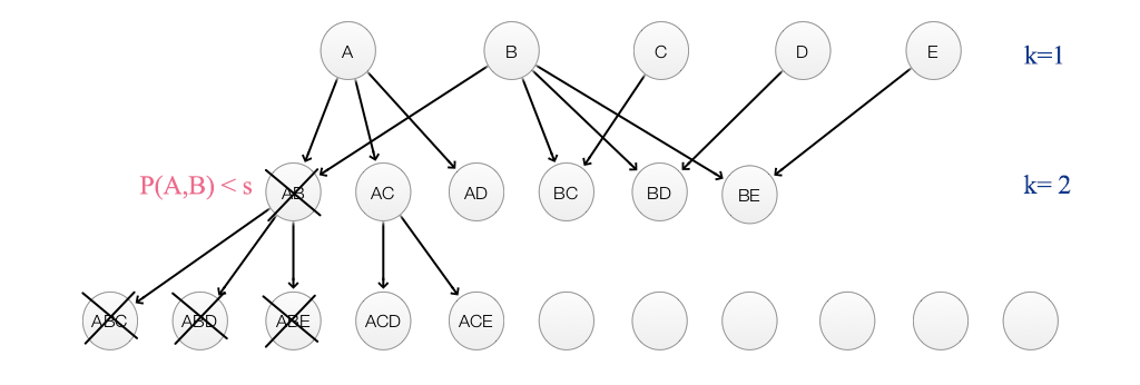
- Generate list of all sets ‘S’ with k = 1.
- Prune candidates where \(p(S) \lt s\)
- Go to k = k + 1 and generate the list again without the pruned items
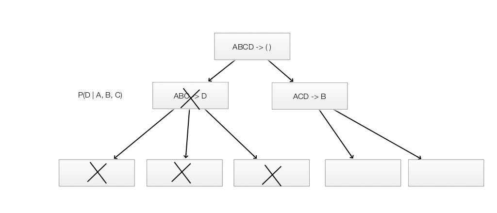
Generating rules
If \(S = {A,B,C}\), we generate candidate rules with all possible sub-sets:
\[\begin{split} & A \implies B, C \quad B \implies A, C, \quad C \implies A, B, \quad \\ & A, B \implies C, \quad A, C \implies B, \quad B, C \implies A. \end{split}\]Once again, we use pruning to reduce the number of evaluation.
Note:
With large amount of data, it is possible that we generate a rule with high probability\(P(S \vert T)\) but yet \(S\) and \(T\) has no special co-relationship. For example, if \(P(T)\) is very high, the corresponding \(P(S \vert T)\) can be pulled above the confidence threshold just because how common \(T\) is.
Lift
One alternative to confidence is lift:
\[Lift(S \implies T) = \frac{P(T \vert S)}{P(T)}\]which reduce the rule likeliness when \(P(T)\) is high.
Clustering
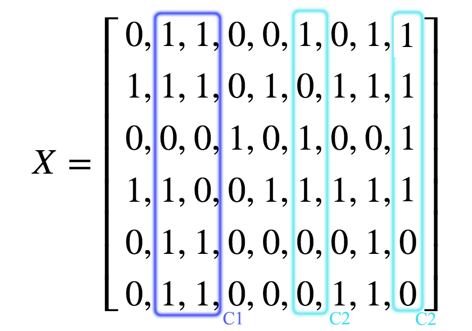
We build a matrix \(X\) containing information on what products users purchase.
Rows in \(X\) contains what a user purchase:
\[X = \begin{bmatrix} -- \text{ Products purchased by user 1 }-- \\ -- \text{ Products purchased by user 2 }-- \\ \cdots \\ -- \text{ Products purchased by user N } -- \\ \end{bmatrix}\]Columns in \(X\) contains who purchase a product:
\[X^T = \begin{bmatrix} -- \text{ Users purchase product 1 }-- \\ -- \text{ Users purchase product 2 }-- \\ \cdots \\ -- \text{ Users purchase product N }-- \\ \end{bmatrix}\] \[X_{ij} = \begin{cases} 1 \text{ User i purchase product j} \\ 0 \text{ otherwise} \end{cases}\]The column \(j\) in \(X\) is the list of users that purchase product \(j\). We can apply clustering to group products (columns) together with the assumption that products are similar if they are purchased by similar users.
We can apply the association rules to make product recommendations.
\[P(T \vert S) > s\]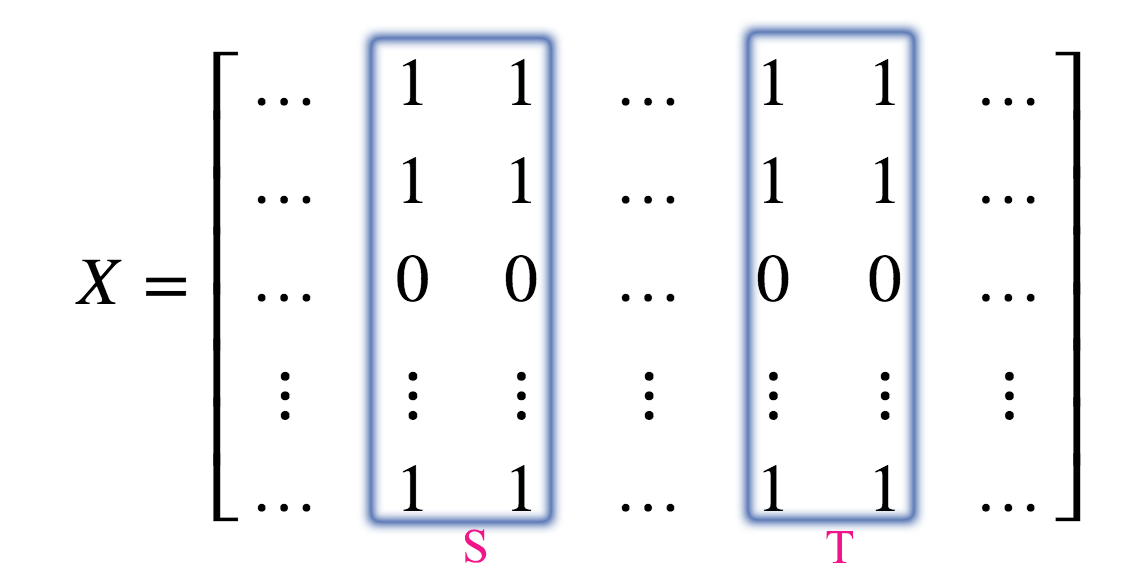
Note: The columns here is the same as the bags of customer in the Amazon recommendation algorithm.
Amazon recommendation algorithm
We need a scalable solution to handle large amount of users and products. First, we can limit the size of \(S\) and \(T\) to 1. Then we compute the similarity of 2 products by:
- Use bag of customer to represent who brought \(item_i\)
| User 1 | User 2 | … | User N | |
| \(X_i\) Item i | 1 | 0 | … | 1 |
| \(X_j\) Item j | 0 | 0 | … | 1 |
- Measure the similarity of 2 items by:
Then we can recommend products by soving the k-nearest neighbors using the cosine similarity as distance measurement.
Content-based filtering
In movie rating, content-based filtering is a supervised learning to extract the genre of a movie and to determine how a person may rate the movie based on its genre. For example, we may define the genre of a movie as:
\[x = (romance, action, scifi)\]We apply supervised learning to learn the genre of a movie say from its marketing material. For example, the genre of a romantic movie can be calculated as:
\[w_j = (1, 0, 0)\]Then we can learn how a person rate a movie based on the type of genre. For example, a person have a 0.9 chance of giving high marks to action or SciFi movies but no chance for romance movies. The preference \(x_i\) for this person will be:
\[x_i = (0, 0.9, 0.9)\]Content-based filtering builds a model to predict rating or recommendation \(y\) given \(x_i\) of a person and \(w_j\) for a movie.
\[y = w^T x \\\]Content-based filtering looks simple but very hard in practice. Collect labels for the training data is hard. Just using the genre to classify a movie may be over simplify on why a person like a movie. We can add more features but what to add becomes very hard.
Collaborative Filtering
Collaborative filtering is an unsupervised learning which we make predictions from ratings supplied by people. Each rows represents the ratings of movies from a person and each column indicates the ratings of a movie.
\[Y = \begin{bmatrix} ? & 1 & 3 & 1 & 5 & ? & \dots & 4 & 1 \\ 2 & 4 & ? & 1 & ? & 3 & \dots & 1 & 2\\ 2 & 3 & 3 & ? & 5 & 1 & \dots & ? & 1\\ & & \vdots & \vdots & \ddots & \vdots & \vdots & \\ ? & 1 & 5 & ? & 4 & ? & \dots & 2 & 1 \\ \end{bmatrix}\]In content-based filtering, we define the feature set \(x = (romance, action, scifi)\) and we recall that the rating can be computed as:
\[y = w^T x \\\]In Collaborative Filtering, we do not know the feature set before hands. Instead, we try to learn those. Just like the handwritten digit recognition MNist, we do not know what features to extract at the beginning but eventually the program learns those latent features (edge. corner, circle) itself.
So let say the latent features that a program learn for a person \(i\) is \(z_i\) and that for a movie \(j\) is \(w_j\). The rating \(y_{ij}\) for the movie will be
\[y_{ij} = w^T_j z_i \\\]Low rank matrix factorization
We are given a matrix \(Y\) which the rows represent people and the columns represent products. Low rank matrix factorization means we decompose the matrix \(Y\) into 2 lower rank matrices: one representing the latent features of \(n\) person and the second represent the latent features of \(m\) products.
\[y_{ij} \approx w^T_j z_i \\\] \[Y = \begin{bmatrix} y_{11} & y_{12} & y_{13} & ? & ? & \dots & y_{1m} \\ y_{21} & y_{22} & ? & y_{24} & ? & \dots & ? \\ & & \vdots & \vdots& \ddots & \vdots & \vdots & \\ y_{n1} & ? & y_{n3} & ? & y_{n5} & \dots & y_{nm} \\ \end{bmatrix} \approx \begin{bmatrix} z_{11} & z_{12} & z_{13} & \dots & z_{1k} \\ z_{21} & z_{22} & z_{23} & \dots & z_{2k} \\ & & \vdots & \ddots & \vdots & \\ z_{n1} & z_{n2} & z_{n3} & \dots & z_{nk} \\ \end{bmatrix} \begin{bmatrix} w_{11} & w_{12} & w_{13} & \dots & w_{1k} \\ w_{21} & w_{22} & w_{23} & \dots & w_{2k} \\ & & \vdots & \ddots & \vdots & \\ w_{m1} & w_{m2} & w_{m3} & \dots & w_{mk} \\ \end{bmatrix}^T\]In collaborative filtering
- We decide the number of latent features to learn. i.e. the dimension of \(w\) and \(z\). More latent features helps us to build a more complex model but will be harder to train.
- Collect data
- User data: User ID, Movie ID, Rating
- Normalize the rating to be zero centered
- Define the cost function as mean square error MSE with L2-regularization
- Optimize \(W\) and \(Z\) using Gradient descent
To find similar products, we can find the similarity between the latent features of two products. \(W\). for example:
\[\| W_i - W_j \|^2\]Bias
We do not need to assume the rating \(y_{ij}\) is zero centered. We can add general bias, bias for the user \(i\) and bias for the product \(j\) in the calculation:
\[\hat{y_{ij}} \approx w^T_j z_i + b + b_i + b_j\\\]Hybrid approach (SVDfeature)
We can also adopt a hybrid approach combing both Collaborative filtering and Content-based filtering. The rating is calculated by combining the ratings from both methods:
\[\hat{y_{ij}} = w^T_j z_i + w_{j}^Tx_{i} + b + b_i + b_j\\\]Explicit vs. implicit feedback
One common approach for the collaborative filtering treats the entries in the user-product matrix as explicit preferences given by the user to a product, for example, users ratings on products. Alternatively, some implicit feedback (like views, clicks, shares etc.) are more widely available. For example in Spark MLlib, it can model collaborative filtering with explicit or implicit feedback. In implicit feedback, MLlib treats the data as the strength of user actions (such as the number of clicks). These numbers are then used in place of the explicit ratings.
The documentation to create a collaborative filtering using MLlib with explicit and implicit feedback can be found in [https://spark.apache.org/docs/latest/mllib-collaborative-filtering.html]
Other recommendation consideration
- New content
- May want to suggest something new or different
- How long should we show the recommendation if user show or do not show interests
- Give editorial recommendation
- Get recommendation from friends or communities
Ranking
Probability ratio for logistic regression
Logistic regression
\[\begin{split} p(y_i \vert x_i, w) & = \frac{1}{1 - e^{-\frac{1}{2}y_i w^T x_i}} \\ & \propto e^{\frac{1}{2}y_i w^T x_i} \\ \end{split}\]Probability ratio for predicting \(y_i\) over \(-y_i\):
\[\begin{split} \frac{p(y_i \vert x_i, w)}{p(- y_i \vert x_i, w)} & \geq \beta \\ \frac{e^{\frac{1}{2}y_i w^T x_i}}{e^{-\frac{1}{2}y_i w^T x_i}} & \geq \beta \\ e^{y_i w^T x_i} & \geq \beta \\ y_i w^T x_i & \geq \log(\beta) \\ y_i w^T x_i & \geq 1 \quad \text{set } \log(\beta)=1\\ \end{split}\]We can define a lost function by the amount of constraint violation:
\[max(0, 1 - y_i w^T x_i )\]Note: This is the Hinge loss and we have proven it from the perspective of probability ratio and constraint violation.
Relevance Ranking
We want to rank the relevance of \(y_i\) based on a query \(x_i\).
\[p(y_i = c \vert x_i, w) \propto e^{w_c^Tx_i}\] \[\begin{split} \frac{p(y_i \vert x_i, w)}{p(y_i = c' \vert x_i, w)} & \geq \beta\\ w_{y_i}^Tx_i - w_{c'}^Tx_i & \geq 1\\ \end{split}\]We can create a cost function based on all constraint violations as:
\[\sum_{i=1}^n max(0, 1 - w_{y_i}^Tx_i + w_{c'}^Tx_i )\]Or a cost function to penalize the highest alternatives:
\[\max_{j \neq i} (max(0, 1 - w_{y_i}^Tx_i + w_{c'}^Tx_i))\]Pairwise ranking
We can rank \(x_i\) and \(x_j\) using probability ratio.
\[p(x_i \vert w) \propto e^{w^Tx_i}\] \[\begin{split} \frac{p(x_i \vert w)}{p(x_j \vert w)} & \geq \beta \quad \text{ for } i \neq j \\ w^Tx_i - w^Tx_j & \geq 1 \quad \text{ for all } i \neq j \\ \end{split}\]We can create a cost function based on all constraint violations as:
\[\sum_{i=1}^n max(0, 1 - w^T x_i + w^T x_j )\]Generalization
We can expand our approach beyond linear regression:
- Define constraint based on probability ratio
- Minimize violation of logarithm of constraint
For pairwise relevance
\[J(w) = \sum_{y_i > y_j} max(0, 1 - \log{ p(y_i \vert w)} + \log{ p(y_j \vert w)}) + \sum^d_{j=1} - \log{p(w_j \vert \lambda) })\]PageRank
Random walk view
- Start at a random webpage
- Follow a random link in each iteration \(t\)
- PageRank is the probability of landing on a page when \(t \rightarrow \infty\)
- Random walk may stuck in part of the graph or never reach some webpage
Damped PageRank algorithm
- Start at a random webpage.
- With the probability \(\epsilon\), go to a random webpage. Otherwise, follow a random link on the page.
- Keep the iteration and compute the probability of landing on a page.