“Machine learning - Regression, Logistic regression, SVM, MAP and Kernels”
Linear regression
\[\begin{split} y & = w^T x \\ y_i & = \sum^k_{j=1} w_j x_{ij} \end{split}\]We transpose \(w\) because by convention we express all vectors as column vectors here.
Mean square error (MSE)
\[\begin{split} J(w) & = \frac{1}{2} \sum^N_{i=1} (w^T x^i - y^i)^2 \end{split}\]which \(x^i\) and \(y^i\) is the input features and the true value for the \(i th\) datapoints in the training dataset.
MSE is popular because it is easy to compute and it has a smooth differentiable To optimize \(w\), we take its differentiate.
\[\begin{split} \nabla_w J & = \sum^N_{i=1} (w^T x^i - y^i) x^i \\ \nabla_w J & = 0 \\ \implies \sum^N_{i=1} (w^T x^i - y^i) x^i & = 0 \\ w^T &= \frac{\sum^N_{i=1} y^i x^i}{\sum^N_{i=1} \| x^i \|^2} \\ \end{split}\]Mean square error (MSE) is actually the L2-norm:
\[L_2 = \| x \|_2\]Since sometimes it is so common, we often drop its subfix.
\[L_2 = \| x \|\]Adding a bias
\[y = w x + b\] \[x = \begin{bmatrix} x^1_1 & x^1_2\\ x^2_1 & x^2_2\\ \end{bmatrix}\]Transform x to:
\[z = \begin{bmatrix} 1 & x^1_1 & x^1_2\\ 1 & x^2_1 & x^2_2\\ \end{bmatrix}\] \[y = w z\]Optimize MSE cost
Here we calculate a generic formula to optimize \(J\).
\[\begin{split} J(w) & = \frac{1}{2} \| xw - y \|_2^2 \\ 2 J(w) & = (xw - y)^T (xw - y) \\ & = (w^Tx^T -y^T) (xw - y) \\ & = w^Tx^T (xw - y) - y^T (xw - y) \\ & = w^Tx^Txw - w^Tx^Ty - y^Txw + y^Ty \\ & = w^Tx^Txw - 2 w^Tx^Ty + y^Ty \\ \text{becase } (y^Txw)^T &= w^T(y^Tx)^T = w^Tx^Ty \\ \end{split}\]Setting \(\nabla_w J = 0\) to optimize \(J\):
\[\begin{split} \nabla_w J = \nabla_w (w^Tx^Txw - 2 w^Tx^Ty + y^Ty) & = 0 \\ \nabla_w (w^Tx^Txw) - 2 \nabla_w (w^Tx^Ty) + \nabla_w (y^Ty) & = 0 \\ \nabla_w (w^T(x^Tx)w) - 2 x^Ty - 0 & = 0 \\ 2 (x^Tx) w - 2 x^Ty - 0 & = 0 \\ (x^Tx) w & = x^Ty \end{split}\]In the following equation, we can solve \(x\) using linear algebra:
\[Ax = b \\\]We will adopt the following notation saying \(x\) is computed by linear algebra using \(A\) and \(b\):
\[x = A \setminus b\]Recall
\[(x^Tx) w = x^Ty\]\(w\) can therefore be solved by:
\[w = x^Tx \setminus x^Ty\]
Notice that the solution for \(w\) are not unique.
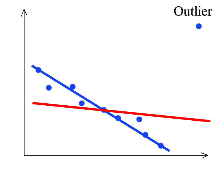
MSE is also vulnerable to outlier. With an outlier, our model is shifted from the blue line to the red line which the blue line can model the training dataset better if the outlier is not there.
L2 regularization with mean square error (MSE)
To avoid overfitting, we use L2-norm as a regularization to the cost function \(J\). (With the MSE computed in the previous section)
\[\begin{split} J(W) & = \frac{1}{2} \| xw - y \|^2 + \frac{\lambda}{2} w^Tw \\ \nabla_w J & = x^Txw - x^Ty + \lambda w \\ \end{split}\]Optimize \(J\):
\[\begin{split} \nabla_w J &= 0 \\ x^Txw - x^Ty + \lambda w &= 0 \\ x^Txw + \lambda w &= x^Ty 0 \\ (x^Tx + \lambda I) w &= x^T y \\ w & = (x^Tx + \lambda I)^{-1} x^T y \end{split}\]With L2 normalization and MSE, \(w\) is:
\[w = (x^Tx + \lambda I)^{-1} x^T y\]
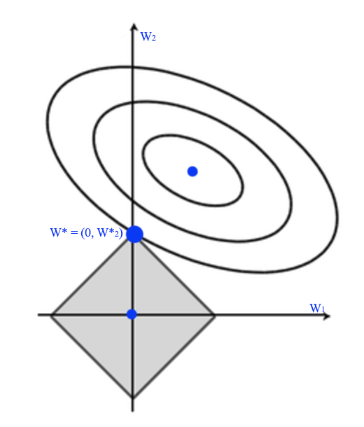
Let’s visualize the solution. In the diagram below, \(W^*_a\) is where regularization cost is 0. i.e. all \(w_i = 0\). \(W^*_b\) is where MSE is minimum. The optimal solution for \(J\) is where the concentric circle meet with the eclipse \(W^*\).
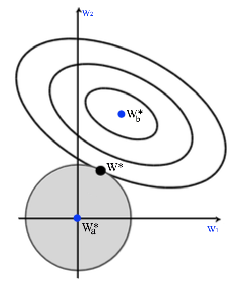
This is also called ridge regression.
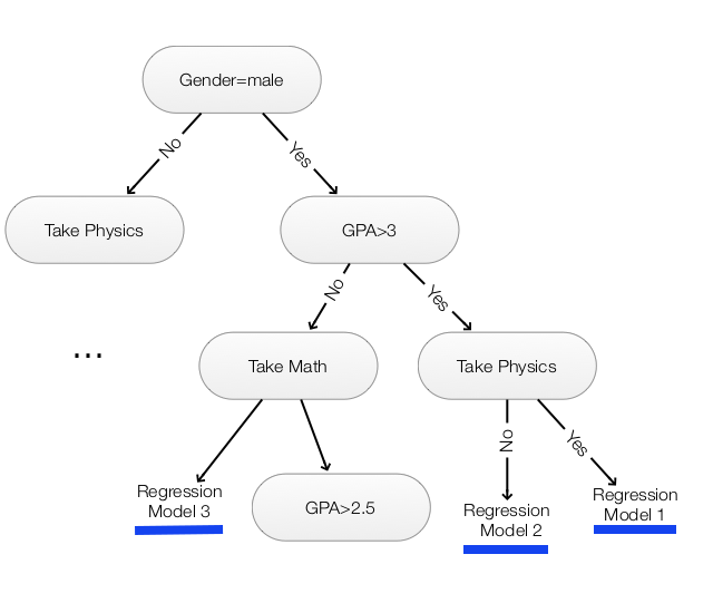
Regression tree
Linear regression models a linear relationship between input and output. We can combine decision tree with linear regression to create a non-linear model.
Change of basis
Non-linearity can be produced by a change of basis also. For example, to model the following quadratic relation:
\[y = w_1 + w_2 x + w_3 x^2\]We can transform \(x\):
\[x = \begin{bmatrix} x^1\\ x^2\\ \cdots\\ \end{bmatrix}\]To:
\[z = \begin{bmatrix} 1 & x^1 & (x^1)^2\\ 1 & x^2 & (x^2)^2\\ & \cdots \end{bmatrix}\]and then apply:
\[y = w z\]To apply a quadratic functions with 2 features:
\[y = w_1 + w_2 x_1 + w_3 x_2 + w_4 x_1 x_2 + w_5 x_1^2 + + w_6 x_2^2\]We transfrom \(x\) to \(z\) with:
\[z = \begin{bmatrix} 1 & x^1_1 & x^1_2 & x^1_1 x^1_2 & (x^1_1)^2 & (x^1_2)^2 \\ 1 & x^2_1 & x^2_2 & x^2_1 x^2_2 & (x^2_1)^2 & (x^2_2)^2 \\ & & & \cdots \end{bmatrix}\]Note: We are not restricted to polynomial functions: any functions including exponentials, logarithms, trigonometric functions can be applied to the basis.
L1-norm as cost functions (Robust regression) or regularization
We are going to explore more cost functions besides MSE. MSE has issues with outliners. It exaggerate the cost by squaring the error. MSE tries harder to fit the outlier into the model. A L1-norm cost function has the same incentive to reduce error from the outlier or a normal data and hence less vulnerable to outlier. Nevertheless, the differential at 0 is not smooth which sometimes impact the effectiveness of the gradient descent in those area.
\[J(w) = \vert xw - y \vert\]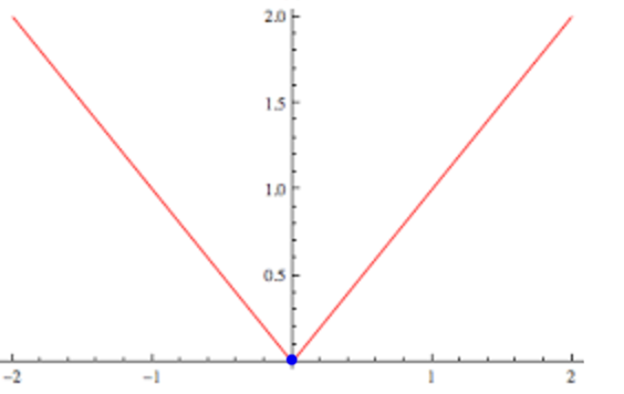
Besides using L-1 as the error cost, L1-norm can be added to the cost function as a regularization, the optimal solution \(w^*\) for the L1 regularization usually push some of the \(w_i\) to be exactly 0.
L1-norm or L1 regularization promotes sparsity for \(w\) which can be desirable to avoid overfitting in particular when we have too many input features. Alternatively, L1-norm can be used for feature selection by eliminate features with \(w_i=0\).
Huber loss
Huber loss smoothes the cost function when \(w\) approach 0 so it is differentiable.
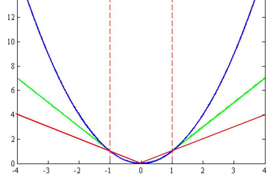
\[\begin{split} J(w) & = \sum^N_{i=1} h(w^Tx^i - y^i)\\ h(r_i) & = \begin{cases} \frac{1}{2} r_i^2 \text{ for } \vert r_i \vert \leq \epsilon \\ \epsilon (\vert r_i \vert - \frac{1}{2} \epsilon) \text{ otherwise} \end{cases} \end{split}\]The blue curve is the MSE, the red is L1-norm and the green is the Huber loss which tries to smooth out at \(w=0\).
L0-norm as regularization
We can add a L0 norm to the regularization. L0-norm even favor more sparsity in \(w\) than L1-norm.
\[L_0 = \| w \|_0 = \begin{cases} 0 \quad \text{ if } w_i = 0 \\ 1 \quad \text{otherwise} \end{cases}\]For example, if \(w=(1, 2, 0, 0, 1)\), the L0-norm regularization is 3.
Since training data is not unlimited, even a true model may have \(w_i=0\), the MSE cost \(\sum^N_{i=1} \| w^Tx -y \|^2\) is likely not bottom at \(w_i=0\). When we add L0 regularization, we add a constant \(\lambda\) to the MSE cost except at \(w_i=0\) which has 0 regularization cost. The total cost shift upward to the green line with the exception at the green dot which remain unchanged.
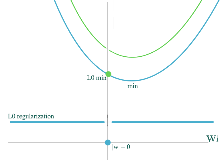
Without regularization, the optimized \(w\) is at the orange dot. With L2 regularization, we may shift the orange dot slightly to the left. However, with a L0 regularization, we can move the optimal point to the green dot subject to the value of \(\lambda\).
Marginal loss (Hinge loss)
Let’s consider a problem to create a boundary to separate the green and red dots below. With a linear regression with MSE cost function, we create a red line to divide the green dots from the red dots. If \(wx_i - y_i > 0\), it is classified as green. As shown 3 green dots will be mis-classified.
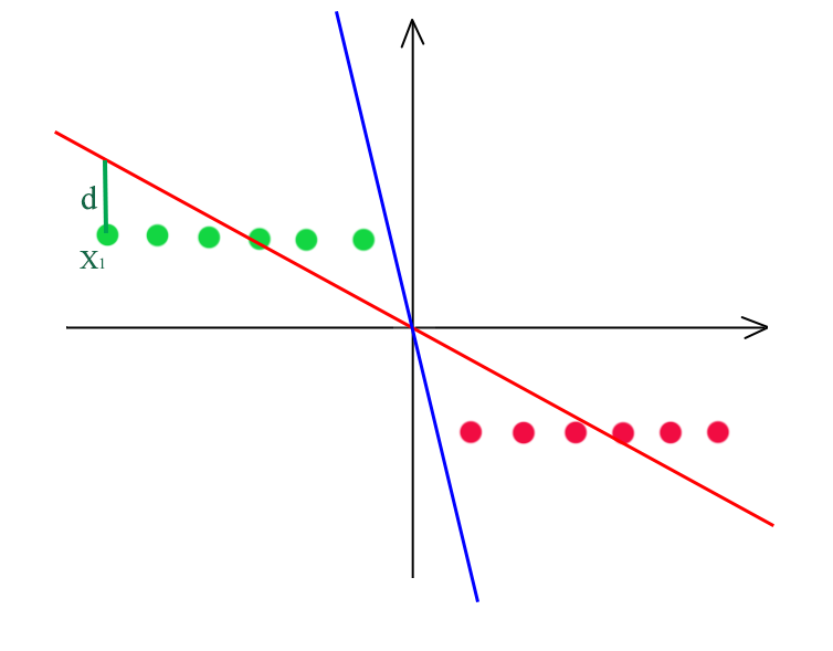
MSE cannot provide an optimal solution (the blue line) because it mis-calculates the cost value. At point \(x_i\), it should be already classified correctly but yet it contributes \(d^2\) to its cost function. Hence, for classification problem, we need a cost function that does not penalize when a good decision is make.
For example, for the green dots, if \(wx_i \geq 1\), the penalty should be set to 0 and we start counting penalty when \(wx_i < 1\).
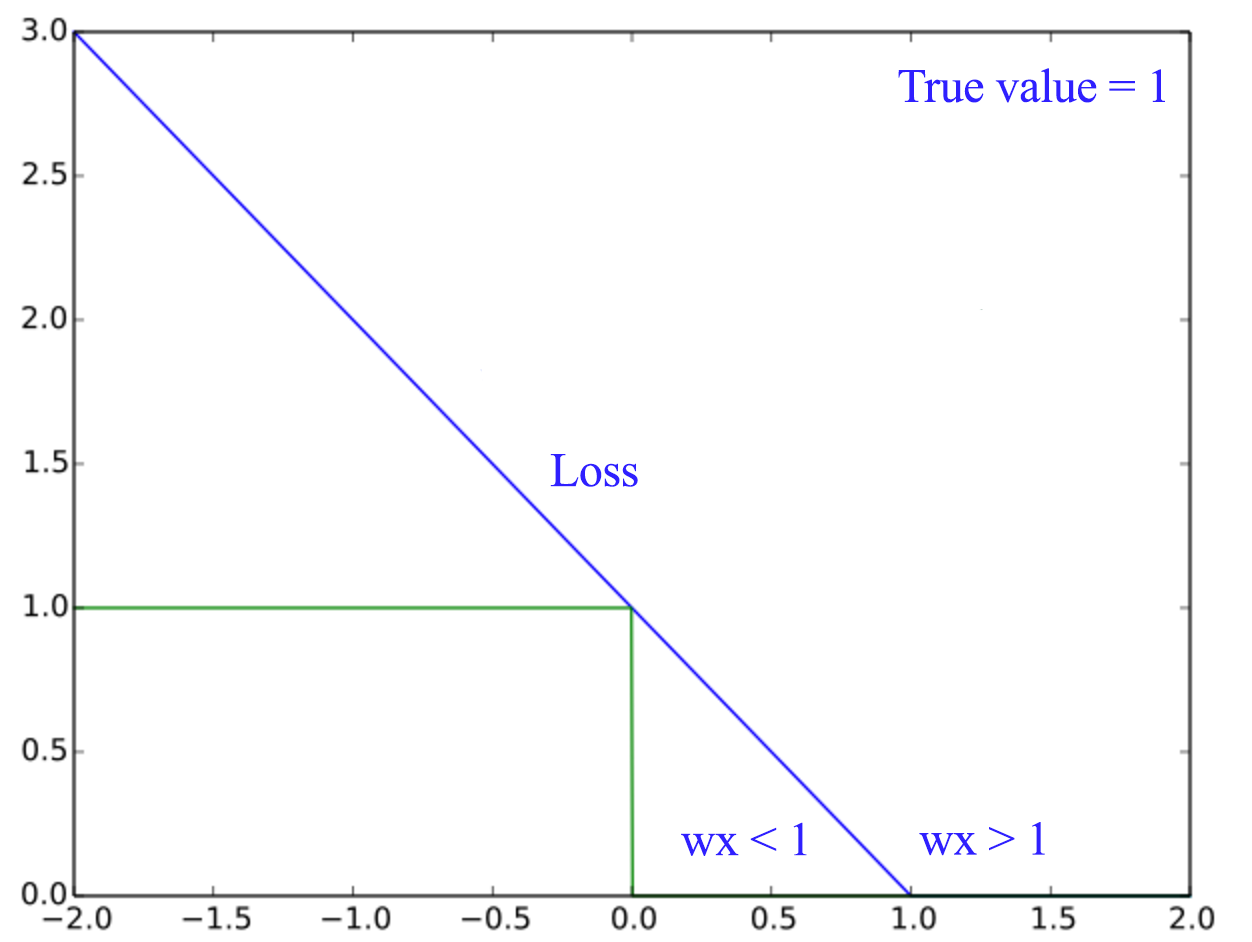
The mathematical equation for Hunge loss is formated as:
\[J(W) = \sum^N_{i=1} max(0, 1 - y^i wx^i)\]Support vector machine (SVM)
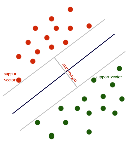
L2-regularization with hinge loss is SVM.
\[\begin{split} J(W) & = \sum^N_{i=1} max(0, 1 - y^i wx^i) + \frac{\lambda}{2} w^T w \\ \end{split}\]The datapoint closest to the gray lines are called support vectors. The optimal solution for SVM maximizes the margins between the support vectors. i.e. SVM creates the largest margin to separate both classes.
We add penalty to the cost function for points where \(y^i wx^i < 1\). i.e. points falls within the max magin.
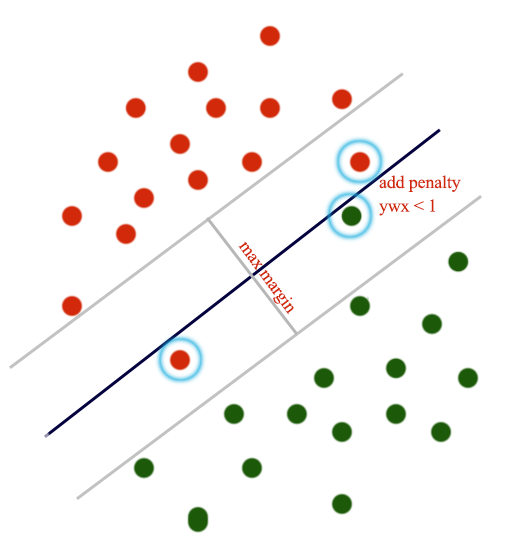
The cost function is defined as the amount of constraint violation.
To have the lowest cost, we want \(w \cdot x > 1\) with the smallest \(\| w\|\). (Assume \(y=1\), \(y= -1\) behave the same way.) The cost is reduced to:
\[\begin{split} J(W) & = \sum^N_{i=1} max(0, 1 - y^i wx^i) + \frac{\lambda}{2} w^T w \quad \quad( \frac{\lambda}{2} \| w\| ) \\ \end{split}\]The dot product of \(w\) and \(x\) is the projection of \(w\) on \(x\). i.e. the green line.
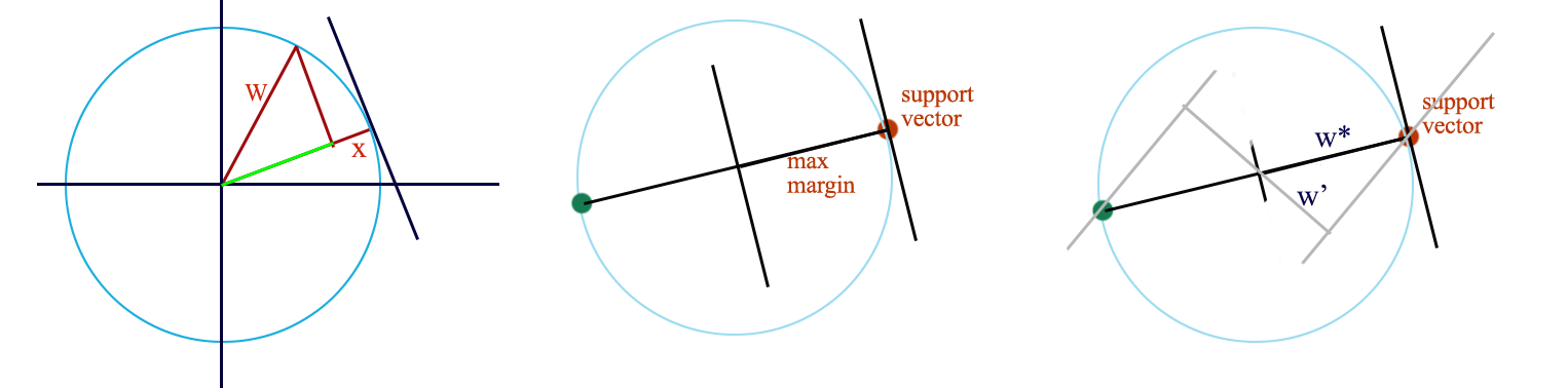
For \(w \cdot x\) to have the maximum value (longest green line), the optimal \(w^{*}\) and \(x\) should be the same. If your draw 2 parallel boundaries passing the support vectors, like the one above on the right, the one with the maximum margin is the radius i.e. \(w^{*}\). Hence the optimal \(w^{*}\) provides the maximum margin for the support vectors. Therefore SVM indeed maximizes the margin.
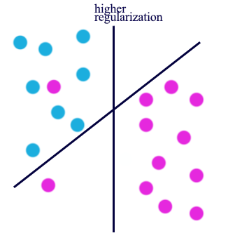
With regularization, we can prevent overfitting for outlier:
\[\begin{split} J(W) & = \sum^N_{i=1} max(0, 1 - y^i wx^i) + \frac{\lambda}{2} w^T w \\ \end{split}\]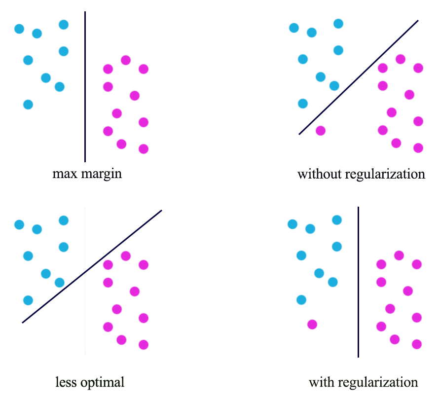
Having different value of regularization level controlled by \(\lambda\), we can have very different optimal solution:
Maximum likelihood estimation
Given a model parameterized by \(w\) and a datapoint \(x_i\), the probability that the model predicts the true value \(y_i\) is:
\[p(y_i \vert x_i, w)\]The probability to match the predictions for all training datapoints become:
\[\begin{split} P(Y \vert X, w) & = \prod^n_{i=1} P( y_i \vert x_i, w) \end{split}\]In our training, we want to find \(w\) that have the highest \(P(Y \vert X, w)\). i.e. we want \(w\) to have the maximum likelihood given our observed training data.
\[w^* = \arg\max_w P(Y \vert X, w)\]Negative log likelihood (NNL)
Logarithm is monotonic. Hence, to maximize a probability function is the same as minimize the negative log of the function.
\[\arg\max_w P(Y \vert X, w) = \arg\min_w - \log(P(Y \vert X, w))\] \[\begin{split} P(Y \vert X, w) & = \prod^n_{i=1} P( y_i \vert x_i, w) \\ -\log(P(Y \vert X, w)) & = - \log \prod^n_{i=1} P( y_i \vert x_i, w) \\ NNL &= - \sum^n_{i=1} \log P( y_i \vert x_i, w) \end{split}\]In later section, NNL is very handy as a cost function because the log cancels the exponential function used in the classifier.
\[NNL = - \sum^n_{i=1} \log P( y_i \vert x_i, w)\]
Linear regression with gaussian distribution
We want to optimize \(\theta\) for a linear regression model with the assumption that \(y\) is gaussian distributed with \(\mu = x\theta\):
\[y_i \sim \mathcal{N}(x_i^T\theta, \sigma^2) = x_i^T\theta + \mathcal{N}(0, \sigma_2)\]Likelihood:
\[\begin{split} p(y \vert x, \theta, \sigma) & = \prod_{i=1}^n p(y_i \vert x_i, \theta, \sigma) \\ & = \prod_{i=1}^n (2 \pi \sigma^2)^{-1/2}e^{- \frac{1}{2 \sigma^2}(y_i - x^T_i \theta)^2} \\ & = (2 \pi \sigma^2)^{-n/2}e^{- \frac{1}{2 \sigma^2} \sum^n_{i=1}(y_i - x^T_i \theta)^2} \\ & = (2 \pi \sigma^2)^{-n/2}e^{- \frac{1}{2 \sigma^2} (y - x \theta)^T(y - x \theta)} \\ \end{split}\]Optimize \(\theta\) using the log likelihood \(l\):
\[\begin{split} J(\theta) & = \log(p(y \vert x, \theta, \sigma)) \\ & = -\frac{n}{2} \log(2 \pi \sigma^2) - \frac{1}{2 \sigma^2}(y - x \theta)^T(y - x \theta) \\ \\ \nabla_\theta J(\theta) & = 0 - \frac{1}{2 \sigma^2} [0 - 2 x^Ty + 2x^Tx\theta] = 0\\ \hat\theta & = (x^Tx)^{-1}x^Ty \end{split}\]The inverse of \(x\) may not be well conditioned. We can add a \(\delta\) to improve the solution:
\[\begin{split} \hat\theta & = (x^Tx)^{-1}x^Ty \\ \hat\theta & = (x^Tx + \delta^2 I )^{-1}x^Ty \\ \end{split}\]Solution:
\[\theta^* \begin{split} = (x^Tx + \delta^2 I )^{-1}x^Ty \\ \end{split}\]
In machine learning, we often use Mean Square Error (MSE) with L2-regularization as our cost function. In fact, the L2-regularization is not a random choice. Here, we proof that solving the equation below lead us to the same solution \(\theta^*\) above.
\[\begin{split} J(\theta) &= \text{MSE } + \text{L2-regularization} \\ &= (y -x\theta)^T(y-x\theta) + \delta^2\theta^T\theta \\ \nabla_\theta J(\theta) & = 2 x^Tx\theta - 2x^Ty + 2 \delta^2 I \theta = 0 \\ \implies & (x^Tx + \delta^2 I ) \theta^* = x^Ty \\ \theta^* &= (x^Tx + \delta^2 I )^{-1}x^Ty \\ \end{split}\]As a side note, we can rewrite the regularization as an optimization constraint which the \(\| \theta \|\) needs to smaller than \(t(\delta)\).
\[\min_{\theta^T\theta \le t(\delta)} (y-x\theta)^T(y-x\theta)\]
Bayesian linear regression
To optimize a linear regression, we can also use Bayesian inference. Based on a prior belief on how \(\theta\) may be distributed (\(\mathcal{N}(\theta \vert \theta_0, V_0)\)), we compute the posterior with the likelihood \(\mathcal{N}(y \vert x\theta, \sigma^2 I )\) using Bayes’ theorem:
\[\begin{split} p( \theta \vert x, y, \sigma^2) & \sim \mathcal{N}(\theta \vert \theta_0, V_0) \mathcal{N}(y \vert x\theta, \sigma^2 I ) = \mathcal{N}(\theta \vert \theta_n, V_n) \\ \theta_n & = V_n V^{-1}_0 \theta_0 + \frac{1}{\sigma^2}V_nx^Ty \\ V^{-1}_n & = V^{-1}_0 + \frac{1}{\sigma^2}x^Tx \end{split}\]Comparison between MLE linear regression and Bayesian linear regression
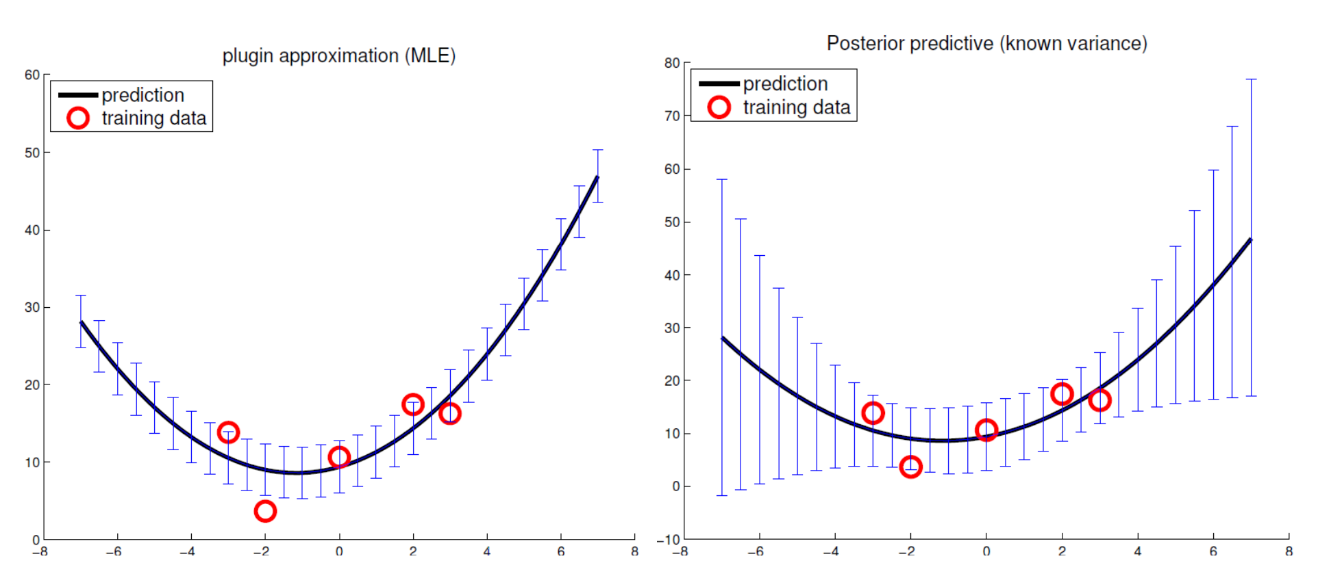
Source Nando de Freitas, UBC machine learning class.
Logistic regression
Logistic function (sigmoid function)
A logistic function is defined as:
\[\begin{split} \sigma(score) & = \frac{1}{1 + e^{-score}} \\ \sigma(wx) & = \frac{1}{1 + e^{-wx}} \end{split}\]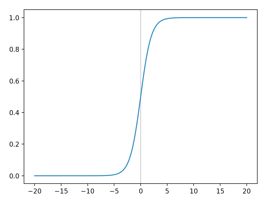
Logistic loss
In a logistic regression, we compute the probability of being a class \(Y\) as:
\[\begin{split} {p(y_{i} | x_{i}, w)} = \sigma(z_{i}) = \frac{1}{1 + e^{-w^Tx}} \end{split}\]Here we use the negative log likeliness (NNL) as our cost function:
\[\begin{split} J_i(W) & = \begin{cases} - \log{ \frac{1}{1 + e^{-w^Tx}}} \quad &\text{ if } y_i = 1 \\ - \log{( 1- \frac{1}{1 + e^{-w^Tx}})} = - \log{ \frac{1}{1 + e^{w^Tx}}} \quad &\text{ if } y_i = -1 \\ \end{cases} \\ J_i(W) &= - \log{ \frac{1}{1 + e^{-yw^Tx}} } \\ J(W) & = \sum^N_{i=1} - \log{ \frac{1}{1 + e^{-yw^Tx}} } \\ & = \sum^N_{i=1} - \log{1} + \log (1 + e^{-yw^Tx}) \\ & = \sum^N_{i=1} \log (1 + e^{-yw^Tx}) \\ \end{split}\]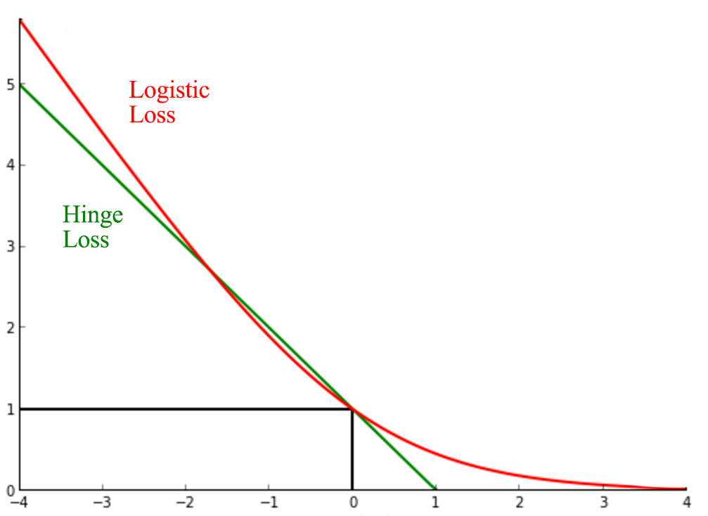
Logistic loss is sometime viewed as the smooth version of the Hinge loss.
Logistic loss with L2 regularization:
\[J(W) = \sum^N_{i=1} \log (1 + e^{-yw^Tx}) + \frac{\lambda}{2} \| w \|^2 \\\]
Maximum a posteriori (MAP)
We use Maximum likelihood estimation as our cost function to find the optimized \(w*\).
\[\begin{split} w^* = \arg\max_w (P(Y \vert X, w)) & = \arg\max_w \prod^n_{i=1} P( y_i \vert x_i, w) \end{split}\]Alternatively, we can use Maximum a posteriori (MAP) to find the optimized \(w*\).
\[P(w \vert x, y)\]In this section, we go through the process of how some cost functions are defined using MAP.
Using Baye’s theorem:
\[\begin{split} p(w \vert x, y) & = \frac{p(y \vert x, w) p(w \vert x)}{p(y \vert x)} \\ & = \frac{p(y \vert x, w) p(w)}{p(y \vert x)} \quad & \text{ w is not depend on x}\\ \end{split}\]Take the negative log
\[\begin{split} -\log p(w \vert x, y) & = - \log p(y \vert x, w) - \log p(w \vert x) - \log p(y \vert x) \\ & = -\log p(y \vert x, w) - \log p(w \vert x) - C^{'} \\ \end{split}\]The total cost for all training data is
\[\begin{split} J(w) & = - \sum^N_{i=1} \log p(y_i \vert x_i, w) - \sum^d_{j=1} \log p(w_j) - C \\ \end{split}\]Compute the prior with the assumption that it has a Gaussian distribution of \(\mu=0, \sigma^2 = \frac{1}{\lambda}\):
\[\begin{split} p(w_j) & = \frac{1}{\sqrt{2 \pi \frac{1}{\lambda}}} e^{-\frac{(w_j - 0)^{2}}{2\frac{1}{\lambda}} } \\ \log p(w_j) & = - \log {\sqrt{2 \pi \frac{1}{\lambda}}} + \log e^{- \frac{\lambda}{2}w_j^2} \\ & = C^{'} - \frac{\lambda}{2}w_j^2 \\ - \sum^d_{j=1} \log p(w_j) &= C + \frac{\lambda}{2} \| w \|^2 \quad \text{ L-2 regularization} \end{split}\]If the likelihood is also gaussian distributed:
\[\begin{split} p(y_i \vert x_i, w) & \propto e^{ - \frac{(w^T x_i - y_i)^2}{2 \sigma^2} } \\ - \sum^N_{i=1} \log p(y_i \vert x_i, w) & = \frac{1}{2 \sigma^2} \| w^T x_i - y_i \|^2 \\ \end{split}\]So for a Gaussian distribution prior and likelihood, the cost function is
\[\begin{split} J(w) & = - \sum^N_{i=1} \log p(y_i \vert x_i, w) - \sum^d_{j=1} \log p(w_j) - C \\ &= \frac{1}{2 \sigma^2} \| w^T x_i - y_i \|^2 + \frac{\lambda}{2} \| w \|^2 + constant \end{split}\]which is the same as the MSE with L2-regularization.
If the likeliness is computed from a logistic function, the corresponding cost function is:
\[\begin{split} p(y_i \vert x_i, w) & = \frac{1}{ 1 + e^{- y_i w^T x_i} } \\ J(w) & = - \sum^N_{i=1} \log p(y_i \vert x_i, w) - \sum^d_{j=1} \log p(w_j) - C \\ &= \sum^N_{i=1} \log(1 + e^{- y_i w^T x_i}) + \frac{\lambda}{2} \| w \|^2 + constant \end{split}\]Softmax classifier
For many classification problems, we categorize an input to one of the many classes. For example, we can classify an image to one of the 100 possible object classes. We use a softmax classifier to compute K probabilities, one per class for an input image (the combined probabilities remains 1).
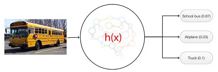
The network computes K scores per image. The probability that an image belongs to the class \(i\) will be.
\[p_i = \frac{e^{score_i}}{\sum e^{score_c}}\]To avoid the numerical stability problem caused by adding large exponential values, we subtract the inputs by its maximum. Adding or subtract a number from the input produces the same probabilities in softmax.
\[softmax(z) = \frac{e^{z_i -C}}{\sum e^{z_c - C}} = \frac{e^{-C} e^{z_i}}{e^{-C} \sum e^{z_c}} = \frac{e^{z_i}}{\sum e^{z_c}}\]Softmax is the most common classifier among others.
Softmax cost function defined as the NLL:
\[\begin{align} J(w) &= - \left[ \sum_{i=1}^{N} \log p(\hat{y} = y \vert x^i, w ) \right] \\ \nabla_{score_{j}} J &= \begin{cases} p - 1 \quad & \hat{y_j} = y \\ p & \text{otherwise} \end{cases} \end{align}\]Non-linear decision boundary
In the classification problem discussed before, classes are separable by a line or a plane. How can we handle non-linear decision boundary?
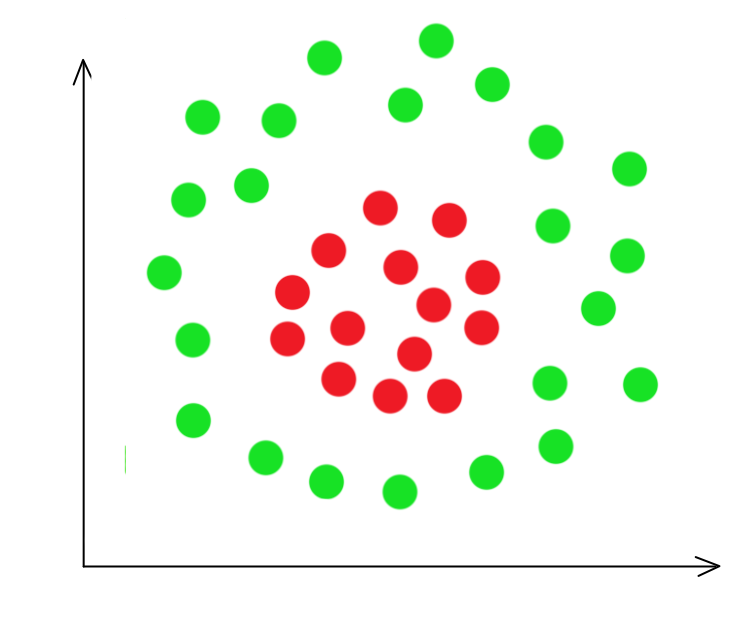
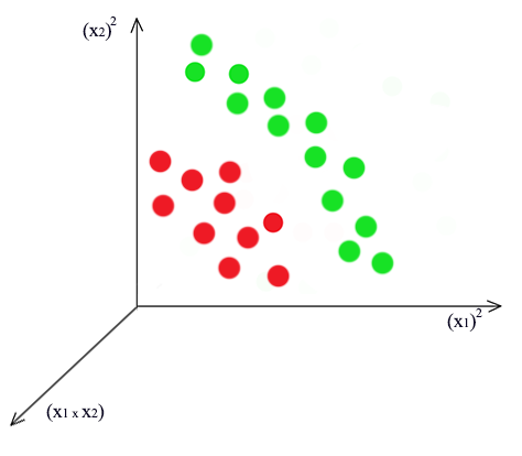
We are changing our basis to a quadric function:
\[z = w_1 x_1^2 + w_2 x_1 x_2 + w_3 x_2^2\] \[z = \begin{bmatrix} 1 & (x^1_1)^2 & x^1_1 x^1_2 & (x^1_2)^2 \\ 1 & (x^2_1)^2 & x^2_1 x^2_2 & (x^2_2)^2 \\ & \cdots \end{bmatrix}\]After the change, we plot it again. It is easy to realize that the \((x_1)^2\) and \((x_2)^2\) plane represent the distance from the center of the cluster and therefore can be divided by a plane.
Other polynomial basis:
\[z = \begin{bmatrix} 1 & x^1_1 & x^1_2 & x^1_1 x^1_2 & (x^1_1)^2 & (x^1_2)^2 \\ 1 & x^2_1 & x^2_2 & x^2_1 x^2_2 & (x^2_1)^2 & (x^2_2)^2 \\ & \cdots \end{bmatrix}\]Recall the optimized \(w\) for a linear regression using MSE + L2 regularization is:
\[\begin{split} w & = (z^Tz + \lambda I)^{-1} z^T y \\ & = z^T (zz^T + \lambda I)^{-1} y \\ \end{split}\]To make a prediction after the change of basis:
\[\begin{split} \hat{y} & = \hat{z}w \\ &= \hat{z} z^T(zz^T + \lambda I)^{-1}y \\ &= \hat{K}(K + \lambda I)^{-1}y) \end{split}\]which the Gram matrix ‘K’ is defined as
\[\begin{split} K & = zz^T \\ & = \begin{bmatrix} (z^1)^T z^1 & (z^1)^T z^2 & \cdots & (z^1)^T z^N \\ (z^2)^T z^1 & (z^2)^T z^2 & \cdots & (z^2)^T z^N \\ & \cdots \\ (z^N)^T z^1 & (z^N)^T z^2 & \cdots & (z^N)^T z^N \\ \end{bmatrix} \end{split}\]which \(K\) contains the inner products between all training examples.
\(\hat{K}\)contains the inner products between test example and training.
Consider a degree 2 basis:
\[x^i = (x^i_1, x^i_2) \\ x^j = (x^j_1, x^j_2) \\\]We change the basis to a quadratic equation:
\[z^i = ((x^i_1)^2, \sqrt{2} x^i_1 x^i_2, (x^i_2)^2) \\ z^i = ((x^j_1)^2, \sqrt{2} x^j_1 x^j_2, (x^j_2)^2) \\\]And K can be computed directly from \(xi\)
\[\begin{split} K = z_i^T z_j &= (x^i_1)^2 (x^j_1)^2 + \sqrt{2} x^i_1 x^i_2 \sqrt{2} x^j_1 x^j_2 + (x^i_2)^2) (x^j_2)^2 \\ &= ( x^i_1 x^j_1 + x^i_2 x^j_2)^2 \\ &= (x^T_i x_j)^2 \end{split}\]Hence, we can compute \(\hat{y}\) from \(x\) directly.
\[\begin{split} \hat{y} &= \hat{K}(K + \lambda I)^{-1}y) \end{split}\]Parametric model vs non-parametric model
A parametric model captures a model with equations and parameters. For example, a linear regression model is represented by a linear equation parameterized by \(w\).
\[y = w^T x\]After a model is built, we make prediction directly from \(w\) and we do not need to keep the training data. If the model is too simple, our predictions will suffer regardless of how big is the training data.
A non-parametric model uses similarity between training data and the testing data to make prediction. The training data becomes the parameters of the model. The K-nearest neighbors classifier is a typical non-parametric model. We locate K nearest neighbors in the training dataset and make predictions based on them. There is little assumption on the model and the predictions improved with the size of the training dataset. A non-parametric model however can be difficult to optimize if the training dataset is too large.
Kernel
Generic form
The generic form of using linear regression with a kernel is:
\[y = b + \sum_i w_i k(x, x^{(i)}).\]which \(x\) contains all \(m\) training datapoints.
There are many kernel functions. For example, using a feature function \(φ\) to extract features:
\[k(x, x^{(i)}) = φ(x) ·φ(x^{(i)})\]Or a Gaussian function to measure the similarity between the training datapoints and the input.
\[k(u, v) = \mathbb{N}(u − v; 0, σ^2)\]Kernel transforms \(x\) non-lineally before applying the linear regression. Therefore, we can take advantage of the convex property of the cost function in linear regression to learn \(w\) efficiently, yet we can transform \(x\) for a non-linear boundary.
Example
In the example below, we use a Gaussian function as a kernel:
\[\begin{split} f_1 && = k(x', x^1) \\ f_2 && = k(x', x^2) \\ \cdots \\ f_n && = k(x', x^n) \\ \end{split}\]which
\[k(x, x^i) = e^{(- \frac{\| x - x^i \|^2}{2 \sigma^2})}\]We use \(y^{(i)}\) as \(w_i\) instead of learning those parameters:
\[\hat{y} = \sum_{i=1}^n y_i f_i\]For example, if we have 3 training datapoints with output \(y^1 = 1, y^2 = -1, y^3 = 1\), then
\[\hat{y} = f_1 - f_2 + f_3\]In classification problem
\[\begin{equation} \hat{y}= \begin{cases} 1 & \text{if } \sum_{i=1}^n y_i f_i \geq 0 \\ -1 & \text{otherwise} \end{cases} \end{equation}\]Radial basis functions (RBF)
Radial basis functions (RBF) is a non-parametric model that use a Gaussian function as a kernel while learning \(w\). In the first step, we build a matrix using all training datapoints (\(x^1, x^2, \cdots x^n\)):
\[z = \begin{bmatrix} k(\| x^1 - x^1 \|) & k(\| x^1 - x^2 \|) & \cdots & k(\| x^1 - x^n \|) \\ k(\| x^2 - x^1 \|) & k(\| x^2 - x^2 \|) & \cdots & k(\| x^2 - x^n \|) \\ \vdots & \vdots & \ddots & \vdots \\ k(\| x^n - x^1 \|) & k(\| x^n - x^2 \|) & \cdots & k(\| x^n - x^n \|) \\ \end{bmatrix}\]which \(k\) is a kernel function to measure similarity between 2 datapoints based on a Gaussian distribution:
\[k(x) = e^{(- \frac{x^2}{2 \sigma^2})}\]and \(w\) is learned from \(z\) and true value \(y\):
\[y = w^T z\]To make prediction for new datapoints \(\hat{x}\):
\[\hat{x} = \begin{bmatrix} \hat{x^1} \\ \hat{x^2} \\ \cdots \\ \hat{x^k} \end{bmatrix}\]We compute \(\hat{z}\):
\[\hat{z} = \begin{bmatrix} k(\| \hat{x^1} - x^1 \|) & k(\| \hat{x^1} - x^2 \|) & \cdots & k(\| \hat{x^1} - x^n \|) \\ k(\| \hat{x^2} - x^1 \|) & k(\| \hat{x^2} - x^2 \|) & \cdots & k(\| \hat{x^2} - x^n \|) \\ \vdots & \vdots & \ddots & \vdots \\ k(\| \hat{x^k} - x^1 \|) & k(\| \hat{x^k} - x^2 \|) & \cdots & k(\| \hat{x^k} - x^n \|) \\ \end{bmatrix}\]The output \(\hat{y}\) is calculated with:
\[\hat{y} = w^T \hat{z}\]If we have only one testing datapoint \(x'\), the equation is simplified to:
\[y = w_1 e^{(- \frac{ \| x' - x_1 \|^2}{2 \sigma^2})} + w_2 e^{(- \frac{ \| x' - x_2 \|^2}{2 \sigma^2})} + \cdots + w_n e^{(- \frac{ \| x' - x_n \|^2}{2 \sigma^2})}\]For example, we have 3 training datapoints \(x_1, x_2, x_3\), each creating a bell curve \(w_1 e^{(- \frac{ \| x' - x_1 \|^2}{2 \sigma^2})}\) indicating how much it contributes to the final output (blue dots) at \(x_i\).
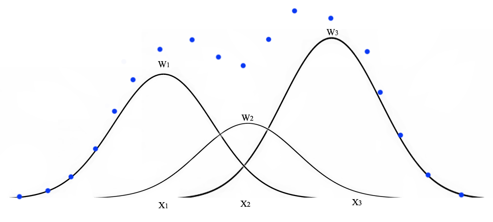
With more datapoints, we can build a complex functions using this gaussian functions.
SVM with kernels
We reuse a Gaussian kernel:
\[\begin{split} x^i \rightarrow \begin{bmatrix} f^i_1 = k( x^i, x_1) & \\ f^i_2 = k( x^i, x_2) & \\ \cdots & \\ f^i_m = k( x^i, x_m) & \\ \end{bmatrix} \end{split}\] \[k(x, x^i) = e^{(- \frac{\| x - x^i \|^2}{2 \sigma^2})}\]Instead of \(y^{(i)}\), we train the model \(w\) with a SVM cost function:
\[\hat{y} = w f\] \[\begin{split} J(W) & = \sum^m_{i=1} max(0, 1 - y^i wf^i) + \frac{\lambda}{2} \| w \|^2 \\ \end{split}\]Choice of \(\lambda\) & \(\sigma\):
- Larger \(\lambda\) means higher regularization. i.e. we want to reduces overfitting. This reduces the variance but increase the bias.
- Larger \(\sigma\) means we take neighbors farther away into consideration. Again, this reduces variance but increases bias.
When to use a linear model (Logistic regression or SVM with linear kernel \(y = w x\) ) or a SVM Gaussian kernel?
Note: N is the number of feature for \(x\) and m is the number of training data.
| N (large) & m (small) | Many input features and vulnerable to overfit with small amount of data | Linear model |
| N (large) & m (large) | Training data is too large to use kernels | Linear model |
| Use non-linear kernel to have a more complex mode | ||
| N (small) & m (large) | Training data is too large to use kernels. Add/Create new features. | Linear model |