“Generative adversarial nets (GAN) , DCGAN, CGAN, InfoGAN”

Discriminative models

In a discriminative model, we draw conclusion on something we observe. For example, we train a CNN discriminative model to classify an image.

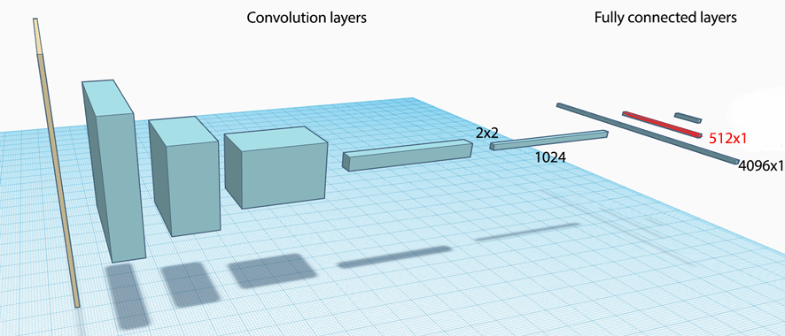
In a previous article on style transfer, we demonstrate how to generate images based on a discriminative model. Basically, we select a specific layer in a CNN, manipulate the gradient manually and backpropagate the gradient to change the image. For example, we want to change an image to make it look similar to another image. We pass the first and the second image to the CNN respectively. We extract the corresponding features of those image at some layers deep down in the network. We manually set the gradient to the difference of the feature values of the images. Then we backpropagate the gradient to make one image look closer to another one.

for t in xrange(num_iterations):
    out_feats, cache = model.forward(X, end=layer)
    dout = 2 * (out_feats - target_feats)    # Manuually override the gradient by the difference of features value.
    dX, grads = model.backward(dout, cache)
    dX += 2 * l2_reg * np.sum(X**2, axis=0)

    X -= learning_rate * dX                  # Use Gradient descent to change the image

We turn around a CNN network to generate realistic images through backpropagation by exaggerate certain features.

Generative models

Discriminative models starts with an image and draw conclusion on something we observe:

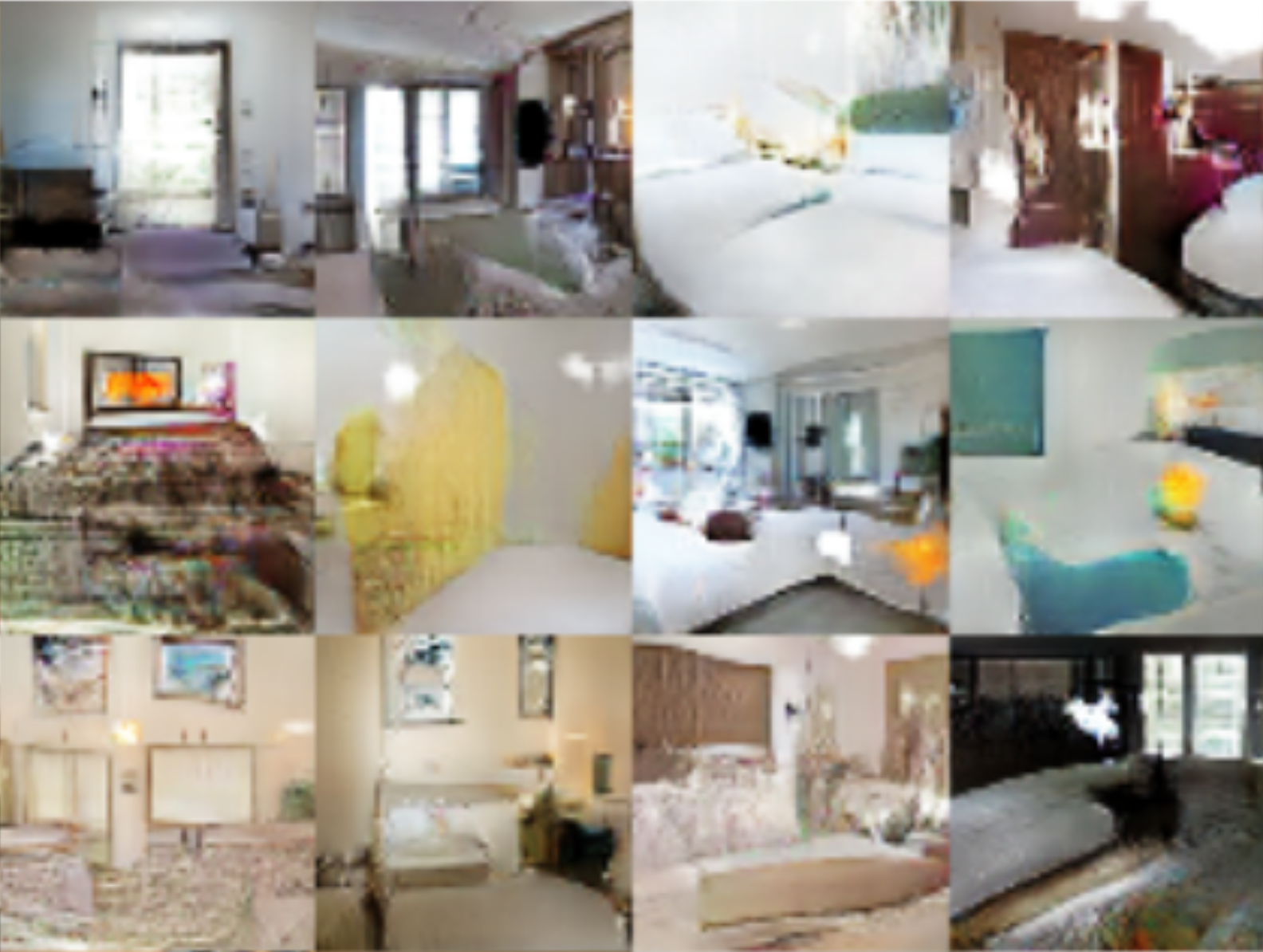
In previous articles, we train a CNN to extract features of our training dataset. Then we start with a noisy image and use backpropagation to make content and style transfer back to the image.

Generative models work in the opposite direction. We starts with some latent representations of the image and generate the image from these variables. For example, we start with some latent variables \(z\) and generate a room picture using a deep network.

Source Alec Radford

Often, we do not know the semantic meaning of the latent variables. i.e. One \(z\) may generate a room with a windo we do not know what the room may look like by just looking at \(z\). In the picture above, we randomly sample 2 different \(z\), say from a uniform distribution or a Gaussian distribution, and 2 different rooms are generated from the generative deep network. As we gradually change \(z\), the room is also gradually changed.

i.e.

Generative adversarial models (GAN) background

Generative adversarial networks compose of 2 deep networks:

• Generator: A deep network generates realistic images.
• Discriminator: A deep network distinguishes real images from computer generated images.

We often compare these GAN networks as a counterfeiter (generator) and a bank (discriminator). Currency are labeled as real or counterfeit to train the bank in identifying fake money. However, the same training signal for the bank is repurposed for training the counterfeiter to print better counterfeit. If done correctly, we can lock both parties into competition that eventually the counterfeit is undistinguishable from real money.

Generator

Given a generator network \(G\) parameterized by \(θ^{(G)}\) and a latent variable \(z\), an image is generated as:

The generator produces images with distribution \(p_{model}(x)\) while the real images have distribution \(p_{data}(x)\).

We can model the discriminator as a classification problem with one data feed coming from real images while another data feed from the generator. The cost function \(J^D\) determines how well that can classify real and computer generated images. We want the probability to be 1 for real image and 0 for computer generated image.

To optimize:

Source Ian Goodfellow

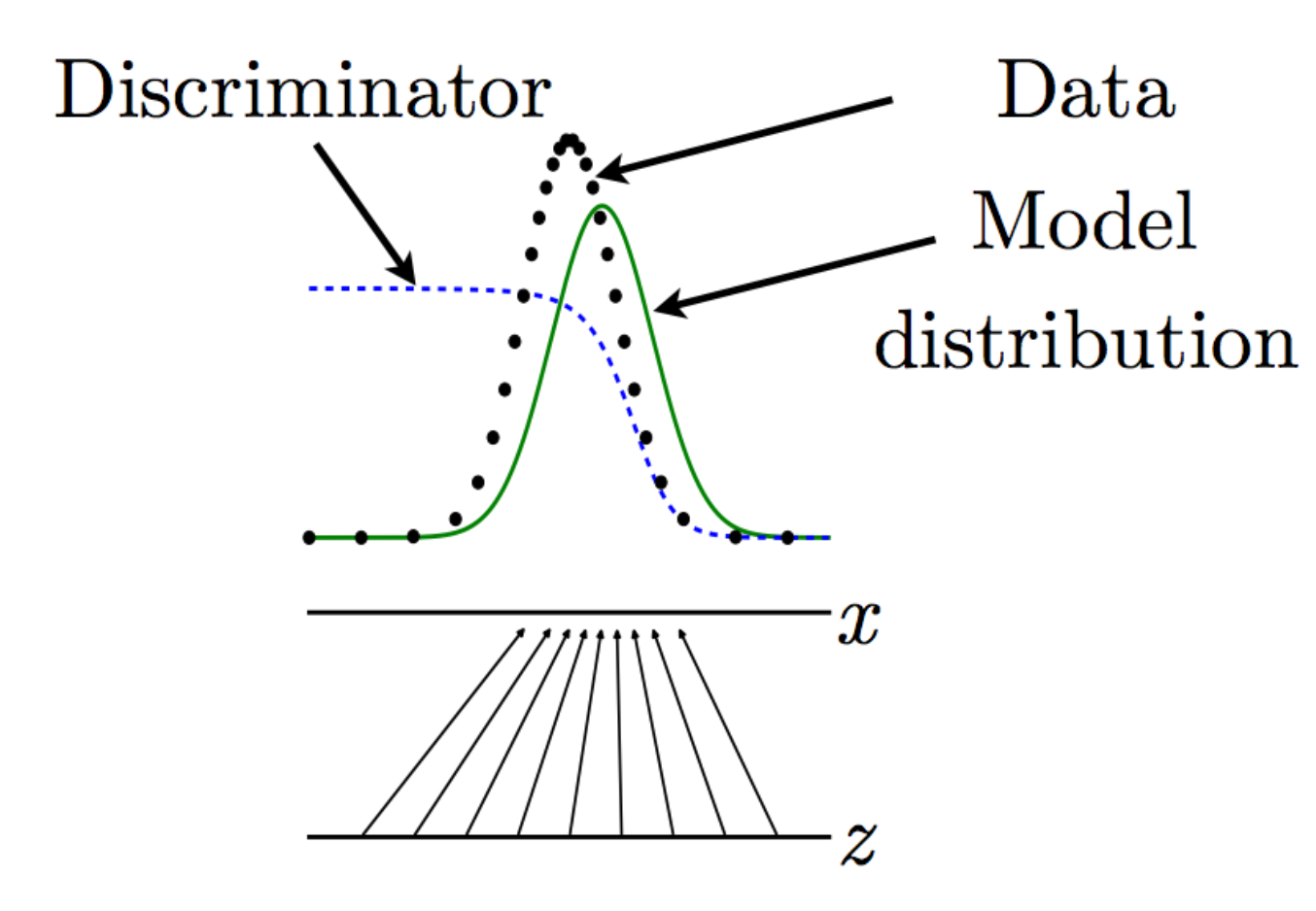
The discriminator (dashed blue line) estimates \(D^{*}(x) = \frac{p_{data}(x)}{p_{data}(x) + p_{model}(x)}\). Whenever the discriminator’s output is high, pmodel(x)pmodel(x) is too low, and whenever the the discriminator’s output is small, the model density is too high. The generator can produce a better model by following the discriminator uphill. i.e. Move G(z) value slightly in the direction that increases D(G(z)).

Zero-sum game (MiniMax)

GAN is a MiniMax game. The generator maximizes the log-probability of labeling real and fake images correctly while the generator minimizes it.

In such a zero-sum game, the generator cost function is defined as the negative of the cost function of the discriminator.

As a zero-sum game, the generator use the negative \(J^{(D)}\) as the cost function. Nevertheless, if the discriminator becomes too accurate, \(J^{(D)} \approx 0\) and therefore the gradient of the generator vanish which make training hard for the generator.

Heuristic, non-saturating game

To resolve that, we can replace the cost function for the generator with:

Maximum likelihood game

We may treat GAN as a maximum likelihood game.

This is equivalent to minimizing:

Comparing cost function

Here is the comparison between 3 different cost function:

Source Ian Goodfellow

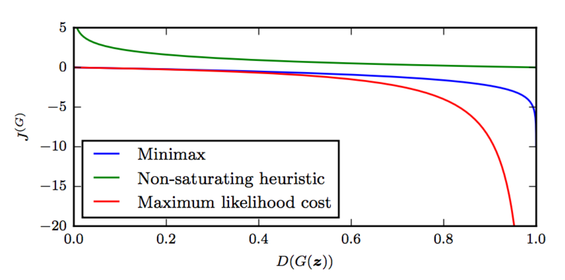
When \(D(G(z)) \approx 0\), the gradient of \(J\) diminishes for MiniMax game and Maximum likelihood game. The generator cannot learn. For Maximum likelihood game, most gradient drops are on the right region. It has very high variance in the cost with most cost gradient coming from samples that the discriminator classified it as real. It means a very small number of samples will dominate the gradient computation for each minibatch.

Nash equilibrium

We can apply Gradient descent to optimize both the generator and the discriminator. However, training GANs requires finding a Nash equilibrium of a non-convex game. Using Gradient descent to seek for a Nash equilibrium may fail: the solution may not converge. i.e. A modification to \(θ^{(D)}\) may reduce \(J^{(D)}\) but increase \(J^{(G)}\) or vice versa. The solution oscillates rather than converges.

To illustrate this, we consider a minimax game between Paul and Mary. Paul controls the value of \(x\) and win the game if \(xy\) is the minimum. Mary controls the value of \(y\) and win the game if \(xy\) is the maximum. The Nash equilibrium defines as a state which all players will not change their strategy regardless of opponent decisions. In this game, the Nash equilibrium is \(x=y=0\). When \(x=0\), Paul will not change the value of \(x\) regardless of how Mary set \(y\). (or vice versa) (1, 1) is not a Nash equilibrium. If \(x=1\), Paul will change \(x\) to negative to win.

The value function is defined as:

Apply gradient descent, the change in parameter \(x\) at each time step is

For Mary:

Combine both equations:

The solution will be:

DCGAN (Deep Convolutional Generative Adversarial Networks)

In DCGAN, we generate an image directly using a deep network while using a second discriminator network to guide the generation process. Here is the generator network:

Source - Alec Radford, Luke Metz, Soumith Chintala:

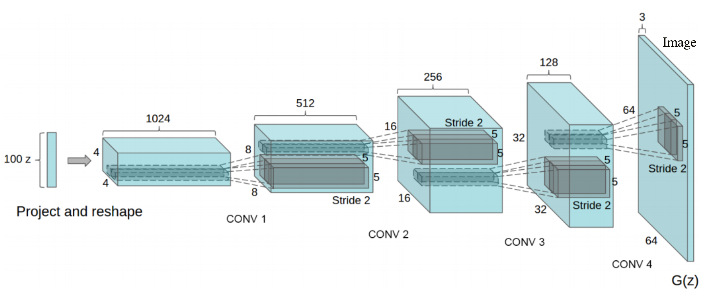
The input \(z\) to the model is a 100-Dimensional vector (100 random numbers). We randomly select input vectors, says \((x_1, x_2, \cdots , x_{100}) = (0.1, -0.05, \cdots, 0.02)\), and create images \(z_{out}\) using multiple layers of transpose convolutions (CONV 1, … CONV 4).

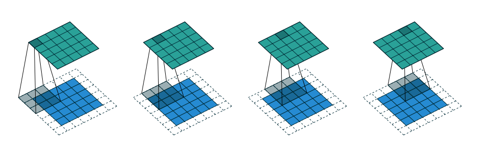
The first animation is the a convolution of a 3x3 filter on a 4x4 input. The second animation is the corresponding transpose convolution of a 3x3 filter on a 2x2 input. Animation source:

5x5 region to a 5x5 region using a 3x3 filter and padding of 1:

2x2 region to a 5x5 region using a 3x3 filter, padding of 1 and stride 2:

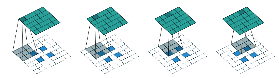
Source: Vincent Dumoulin and Francesco Visin

Transpose convolutions are sometimes call deconvolution.

At the beginning, \(z_{out}\) are just random noisy images. In DCGAN, we use a second network called a discriminator to guide how images are generated. With the training dataset and the generated images from the generator network, we train the discriminator (just another CNN classifier) to classify whether its input image is real or generated. But simultaneously, for generated images, we backpropagation the score in the discimiantor to the generator network. The purpose is to train the \(W\) of the generator network so it can generate more realistic images. So the discriminator servers 2 purposes. It determines the fake one from the real one and gives the score of the generated images to the generative model so it can train itself to create more realistic images. By training both networks simultaneously, the discriminator is better in distinguish generated images while the generator tries to narrow the gap between the real image and the generated image. As both improving, the gap between the real and generated one will be diminished.

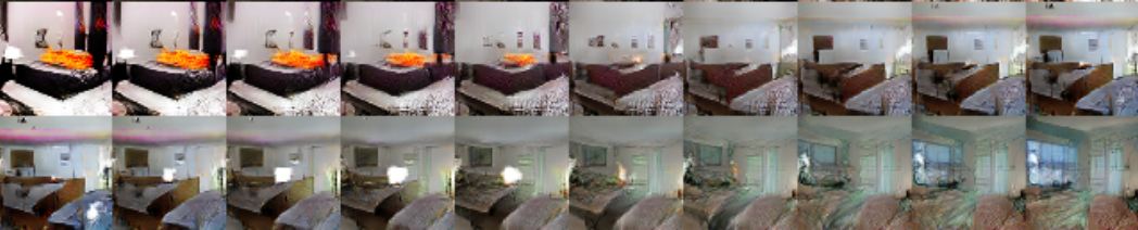
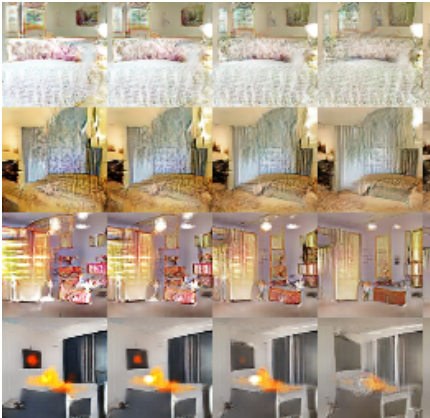
The following are some room pictures generated by DCGAN:

Source - Alec Radford, Luke Metz, Soumith Chintala:

As we change \(z\) gradually, the images will be changed gradually also.

The following code is written in TensorFlow.

Here is a discriminator network that looks similar to the usual CNN classification network. It compose of 4 convolution layers. With the exception of the first convolution layer, other convolution layers are linked with a batch normalization layer and then a leaky ReLU. Finally, it is connected to a fully connected layer (linear) with a sigmoid classifier.

def discriminator(image):
    d_bn1 = batch_norm(name='d_bn1')
    d_bn2 = batch_norm(name='d_bn2')
    d_bn3 = batch_norm(name='d_bn3')

    h0 = lrelu(conv2d(image, DIM, name='d_h0'))
    h1 = lrelu(d_bn1(conv2d(h0, DIM * 2, name='d_h1')))
    h2 = lrelu(d_bn2(conv2d(h1, DIM * 4, name='d_h2')))
    h3 = lrelu(d_bn3(conv2d(h2, DIM * 8, name='d_h3')))
    h4 = linear(tf.reshape(h3, [batchsize, -1]), 1, scope='d_h4')
    return tf.nn.sigmoid(h4), h4

The generator looks very similar to the reverse of the discriminator except the convolution layer is replaced with the transpose convolution layer.

def generator(z):
    g_bn0 = batch_norm(name='g_bn0')
    g_bn1 = batch_norm(name='g_bn1')
    g_bn2 = batch_norm(name='g_bn2')
    g_bn3 = batch_norm(name='g_bn3')

    z2 = linear(z, DIM * 8 * 4 * 4, scope='g_h0')
    h0 = tf.nn.relu(g_bn0(tf.reshape(z2, [-1, 4, 4, DIM * 8])))
    h1 = tf.nn.relu(g_bn1(conv_transpose(h0, [batchsize, 8, 8, DIM * 4], name="g_h1")))
    h2 = tf.nn.relu(g_bn2(conv_transpose(h1, [batchsize, 16, 16, DIM * 2], name="g_h2")))
    h3 = tf.nn.relu(g_bn3(conv_transpose(h2, [batchsize, 32, 32, DIM * 1], name="g_h3")))
    h4 = conv_transpose(h3, [batchsize, 64, 64, 3], name="g_h4")
    return tf.nn.tanh(h4)

We build a placeholder for image to the discriminator, and a placeholder for \(z\). We build 1 generator and initializes 2 discriminators. But both discriminators share the same trainable parameters so they are actually the same. However, with 2 instances, we can separate the scores (logits) for the real and the generated images by feed real images to 1 discriminator and generated images to another.

images = tf.placeholder(tf.float32, [batchsize, DIM, DIM, 3] , name="real_images")
zin = tf.placeholder(tf.float32, [None, Z_DIM], name="z")

G = generator(zin)
with tf.variable_scope("discriminator") as scope:
    D_prob, D_logit = discriminator(images)
    scope.reuse_variables()
    D_fake_prob, D_fake_logit = discriminator(G)

We computed the lost function for the discriminator using the cross entropy for both real and generated images.

d_loss_real = tf.reduce_mean(tf.nn.sigmoid_cross_entropy_with_logits(
                 logits=D_logit, labels=tf.ones_like(D_logit)))
d_loss_fake = tf.reduce_mean(tf.nn.sigmoid_cross_entropy_with_logits(
                 logits=D_fake_logit, labels=tf.zeros_like(D_fake_logit)))
d_loss = d_loss_real + d_loss_fake

We compute the lost function for the generator by using the logits of the generated images from the discriminator. Then, we backpropagate the gradient to train the \(W\) such that it can later create more realistic images.

g_loss = tf.reduce_mean(tf.nn.sigmoid_cross_entropy_with_logits(
                 logits=D_fake_logit, labels=tf.ones_like(D_fake_logit)))

We use 2 separate optimizer to train both network simultaneously:

t_vars = tf.trainable_variables()
d_vars = [var for var in t_vars if 'd_' in var.name]
g_vars = [var for var in t_vars if 'g_' in var.name]

d_optim = tf.train.AdamOptimizer(learningrate, beta1=beta1).minimize(d_loss, var_list=d_vars)
g_optim = tf.train.AdamOptimizer(learningrate, beta1=beta1).minimize(g_loss, var_list=g_vars)

The full source code is available here.

Feature mapping

Avoiding the over training of the discriminator, we have a more refined objective to have the statistics of the features in the generated images to match those of real images in the intermediate layer of the discriminator.

The new cost function for the generator is:

Minibatch discrimination

The discriminator processes each datapoint independently and there is no mechanism to encourage the generator to create more diversify images (the generator may collapse to very similar output). In minibatch discrimination, we add information about its co-relationship with other images as input to the discriminator.

\(f\) be the feature vector of datapoint \(i\) in the intermediate layer of the discriminator. \(T\) is another tensor to train.

We use the following as the input to the next immediate layer:

Minibatch discrimination works better than feature mapping in image generation. But for semi-supervising learning, feature mapping creates better datapoints for the classifier.

Historical averaging

We add the following to each player cost which \(θ[i]\) is the parameter at time \(i\).

The added cost help the gradient descent to find the equilibria of some low-dimensional, continuous non-convex games.

One-sided label smoothing

Sometimes the gradient for the generator can become very large if the discriminator becomes too confident. Adversary networks are vulnerable for such highly confident outputs even the classification is right. One-sided label smoothing regulates the discriminator not to be over confidence. It replaces the 1 targets for a classifier with smoothed values, like 0.9.

Virtual batch normalization (VBN)

Batch normalization subtracts the mean and dividing by the standard deviation of a feature on a minibatch of data. If the sample batch is small, it generates un-expected side effects to the generated images. For example, if one batch of training data has green-tinted while another batch of training data has yellow-tinted area. We see the generator starts create image with both yellow and green-tinted area.

We can compute \(\mu, \sigma\) from a reference batch. However, we may overfit our model with this reference batch sample. VBM compute both value from the minibatch and the reference batch to mitigate the problems.

VBN is expensive and will be used only in the generator network.

Other tips

• Model size: In practice, the discriminator is deeper and sometimes has more filters per layer than the generator.
• Train with labels: Introduce labeling in the generator or having discriminator to recognize specific classes always help image quality.

Conditional Generative Adversarial Nets (CGAN)

In the MNIST dataset, it will be nice to have a latent variable representing the class of the digit (0-9). Even better, we can have another variable for the digit’s angle and one for the stroke thickness. In GAN, the input of the encoder and the decoder are:

In CGAN, we explicitly define \(y\) (the class, the digit’s angle, stroke thickness etc …) as an additional input to the encoder and the decoder

Define the placeholder for \(x, y\) and \(z\). We explicitly use a 1-hot vector of the label (0-9) as y.

X_dim = mnist.train.images.shape[1]   # x (image) dimension
y_dim = mnist.train.labels.shape[1]   # y dimensions = label dimension = 10
Z_dim = 100                           # z (latent variables) dimension

X = tf.placeholder(tf.float32, shape=[None, X_dim])     # (-1, 784)
y = tf.placeholder(tf.float32, shape=[None, y_dim])     # (-1, 10) y: Use a one-hot vector for label 
Z = tf.placeholder(tf.float32, shape=[None, Z_dim])     # (-1, 100) z

Create the generator and discriminator TensorFlow operations. \(G(z,y)\) and \(D(x, y)\).

G_sample = generator(Z, y)
D_real, D_logit_real = discriminator(X, y)
D_fake, D_logit_fake = discriminator(G_sample, y)

Concatenate \(z\) and \(y\) as input to the generator \(G(z, y)\). Code for the generator:

def generator(z, y):
    # Concatenate z and y as input
    inputs = tf.concat(axis=1, values=[z, y])
    G_h1 = tf.nn.relu(tf.matmul(inputs, G_W1) + G_b1)
    ...

The code for the generator:

h_dim = 128

""" Generator Net model """
G_W1 = tf.Variable(he_init([Z_dim + y_dim, h_dim]))
G_b1 = tf.Variable(tf.zeros(shape=[h_dim]))

G_W2 = tf.Variable(he_init([h_dim, X_dim]))
G_b2 = tf.Variable(tf.zeros(shape=[X_dim]))

def generator(z, y):
    # Concatenate z and y as input
    inputs = tf.concat(axis=1, values=[z, y])
    G_h1 = tf.nn.relu(tf.matmul(inputs, G_W1) + G_b1)
    G_log_prob = tf.matmul(G_h1, G_W2) + G_b2
    G_prob = tf.nn.sigmoid(G_log_prob)

    return G_prob

The code for the discriminator:

""" Discriminator Net model """
D_W1 = tf.Variable(he_init([X_dim + y_dim, h_dim]))
D_b1 = tf.Variable(tf.zeros(shape=[h_dim]))

D_W2 = tf.Variable(he_init([h_dim, 1]))
D_b2 = tf.Variable(tf.zeros(shape=[1]))

def discriminator(x, y):
    inputs = tf.concat(axis=1, values=[x, y])
    D_h1 = tf.nn.relu(tf.matmul(inputs, D_W1) + D_b1)
    D_logit = tf.matmul(D_h1, D_W2) + D_b2
    D_prob = tf.nn.sigmoid(D_logit)

    return D_prob, D_logit

Cost function for the discriminator and the generator:

D_loss_real = tf.reduce_mean(tf.nn.sigmoid_cross_entropy_with_logits(logits=D_logit_real, 
                             labels=tf.ones_like(D_logit_real)))   # True label is 1 for real data
D_loss_fake = tf.reduce_mean(tf.nn.sigmoid_cross_entropy_with_logits(logits=D_logit_fake, 
                             labels=tf.zeros_like(D_logit_fake)))  # True label is 0
D_loss = D_loss_real + D_loss_fake

G_loss = tf.reduce_mean(tf.nn.sigmoid_cross_entropy_with_logits(logits=D_logit_fake, 
                             labels=tf.ones_like(D_logit_fake)))   # True label is 1

Create the optimizer for the discriminator and the generator:

D_solver = tf.train.AdamOptimizer().minimize(D_loss, var_list=theta_D)
G_solver = tf.train.AdamOptimizer().minimize(G_loss, var_list=theta_G)

Reading \(x\) and \(y\) and sampling \(z\) for execution:

def sample_Z(m, n):
    return np.random.uniform(-1., 1., size=[m, n])

...

X_data, y_data = mnist.train.next_batch(batch_size)
...

Z_sample = sample_Z(batch_size, Z_dim)
_, D_loss_curr = sess.run([D_solver, D_loss], 
                          feed_dict={X: X_data, Z: Z_sample, y:y_data})
_, G_loss_curr = sess.run([G_solver, G_loss], 
                          feed_dict={Z: Z_sample, y:y_data})

Generate samples from our learned model:

n_sample = 16

Z_sample = sample_Z(n_sample, Z_dim)
y_sample = np.zeros(shape=[n_sample, y_dim])
y_sample[:, 7] = 1   # Only generate the digit 7

samples = sess.run(G_sample, feed_dict={Z: Z_sample, y:y_sample})

Here is the model generated “7”:

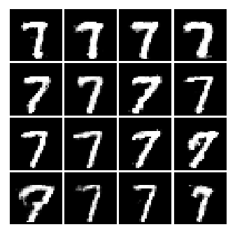
The full source code is in here which is modified from wiseodd.

InfoGAN

In CGAN’s MNIST, we read the labels of the images and explicitly pass it into the generator and discriminator as \(y\).

In InfoGAN, the generator and the discriminator are:

which \(c\) is the latent code representing the semantic features of the datapoints and the noise vector \(z\) is the source of noise for the latent variables similar to CGAN. In InfoGAN, \(c\) will be learned from \(x\) in a deep net instead of initialized it explicitly with labels in CGAN.

Creating a generator and a discriminator

X = tf.placeholder(tf.float32, shape=[None, 784])
Z = tf.placeholder(tf.float32, shape=[None, 16])
c = tf.placeholder(tf.float32, shape=[None, 10])

G_sample = generator(Z, c)
D_real = discriminator(X)
D_fake = discriminator(G_sample)

Generator operations

G_W1 = tf.Variable(he_init([26, 256]))
G_b1 = tf.Variable(tf.zeros(shape=[256]))

G_W2 = tf.Variable(he_init([256, 784]))
G_b2 = tf.Variable(tf.zeros(shape=[784]))

theta_G = [G_W1, G_W2, G_b1, G_b2]

def generator(z, c):
    """
    :param z: (-1, 16)
    :param c: (-1, 10)
    """
    inputs = tf.concat(axis=1, values=[z, c])
    G_h1 = tf.nn.relu(tf.matmul(inputs, G_W1) + G_b1)
    G_log_prob = tf.matmul(G_h1, G_W2) + G_b2
    G_prob = tf.nn.sigmoid(G_log_prob)

    return G_prob

Discriminator operations

D_W1 = tf.Variable(he_init([784, 128]))
D_b1 = tf.Variable(tf.zeros(shape=[128]))

D_W2 = tf.Variable(he_init([128, 1]))
D_b2 = tf.Variable(tf.zeros(shape=[1]))

theta_D = [D_W1, D_W2, D_b1, D_b2]

def discriminator(x):
    """
    :param x: (-1, 784)
    """
    D_h1 = tf.nn.relu(tf.matmul(x, D_W1) + D_b1)
    D_logit = tf.matmul(D_h1, D_W2) + D_b2
    D_prob = tf.nn.sigmoid(D_logit)

    return D_prob

Unlike CGAN, \(c\) is learned from a deep net instead of explicitly define it.

One naive approach is to create a new deep net \(Q\) to approximate \(c\) given \(x\).

# p(c|x) 
Q_W1 = tf.Variable(he_init([784, 128]))
Q_b1 = tf.Variable(tf.zeros(shape=[128]))

Q_W2 = tf.Variable(he_init([128, 10]))
Q_b2 = tf.Variable(tf.zeros(shape=[10]))

theta_Q = [Q_W1, Q_W2, Q_b1, Q_b2]

def Q(x):
    """
    :param x: (-1, 784)
    """
    Q_h1 = tf.nn.relu(tf.matmul(x, Q_W1) + Q_b1)
    Q_prob = tf.nn.softmax(tf.matmul(Q_h1, Q_W2) + Q_b2)

    return Q_prob

Creating the generator and discriminator:

X = tf.placeholder(tf.float32, shape=[None, 784])
Z = tf.placeholder(tf.float32, shape=[None, 16])
c = tf.placeholder(tf.float32, shape=[None, 10])

G_sample = generator(Z, c)
D_real = discriminator(X)
D_fake = discriminator(G_sample)
Q_c_given_x = Q(G_sample)

The loss function for Q is defined as:

cross_ent = tf.reduce_mean(-tf.reduce_sum(tf.log(Q_c_given_x + 1e-8) * c, 1))
ent = tf.reduce_mean(-tf.reduce_sum(tf.log(c + 1e-8) * c, 1))
Q_loss = cross_ent + ent

And the optimizer:

theta_G = [G_W1, G_W2, G_b1, G_b2]
theta_Q = [Q_W1, Q_W2, Q_b1, Q_b2]
theta_Q = [Q_W1, Q_W2, Q_b1, Q_b2]

D_solver = tf.train.AdamOptimizer().minimize(D_loss, var_list=theta_D)
G_solver = tf.train.AdamOptimizer().minimize(G_loss, var_list=theta_G)
Q_solver = tf.train.AdamOptimizer().minimize(Q_loss, var_list=theta_G + theta_Q)

Training:

def sample_Z(batch_size, z_dim):
    return np.random.uniform(-1., 1., size=[batch_size, z_dim])

def sample_c(batch_size):
    return np.random.multinomial(1, 10 * [0.1], size=batch_size)

X_data, _ = mnist.train.next_batch(batch_size)
Z_noise = sample_Z(batch_size, Z_dim)
c_noise = sample_c(batch_size)

_, D_loss_curr = sess.run([D_solver, D_loss],
                              feed_dict={X: X_data, Z: Z_noise, c: c_noise})

_, G_loss_curr = sess.run([G_solver, G_loss],
                              feed_dict={Z: Z_noise, c: c_noise})

sess.run([Q_solver], feed_dict={Z: Z_noise, c: c_noise})

The full source code is in here which is modified from wiseodd.

Cost function

In information theory, the mutual information between \(X\) and \(Y\) is \(I(X; Y )\). It measures how much we will know \(X\) if we know \(Y\) or vice versa. If \(X\) and \(Y\) are independent, \(I(X; Y )=0\)

which \(H\) is the entropy.

Given \(x \sim P_G(x)\), we want \(P_G(c \vert x)\) to have a small entropy. InfoGAN want to solve the minmax of

with

To compute \(I(c \vert x = G(z, c))\), we need to approximate \(p(c \vert x)\) with a function \(Q(c \vert x)\) (Variation Maximization)

Variation Maximization of mutual information

To find the lower bound of \(I\):

Define a variational lower bound:

which \(Q\) is a function approximator for \(p(c \vert x)\). InfoGan minmax the following equation:

Compute \(V_{GAN} (D, G)\) in TensorFlow:

D_loss = -tf.reduce_mean(tf.log(D_real + 1e-8) + tf.log(1 - D_fake + 1e-8))
G_loss = -tf.reduce_mean(tf.log(D_fake + 1e-8))

Compute \(L_I (G, Q)\) in TensorFlow:

cross_ent = tf.reduce_mean(-tf.reduce_sum(tf.log(Q_c_given_x + 1e-8) * c, 1))
ent = tf.reduce_mean(-tf.reduce_sum(tf.log(c + 1e-8) * c, 1))
Q_loss = cross_ent + ent

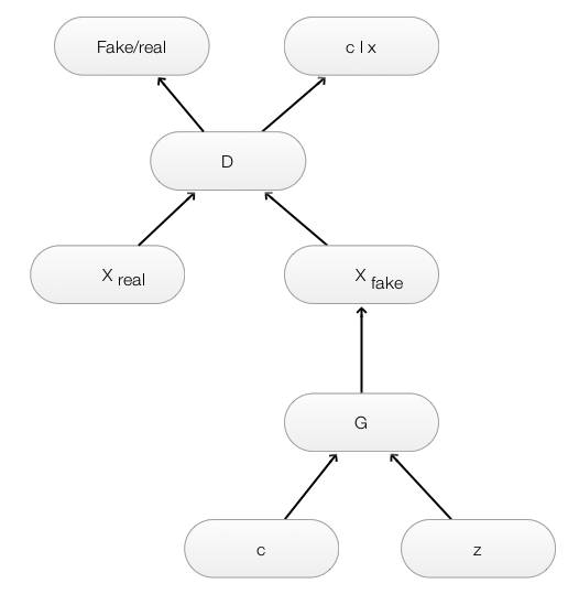
In InfoGAN, we do not create a separate \(Q\) net. Instead, \(Q\) and \(D\) share all CNN layers in the discriminator but with one fully connected layer dedicated to output \(Q(c \vert x)\) from \(x_{fake}\). For latent code \(c_i\), it applies softmax to represent \(Q(c_i \vert x)\). For continuous latent code \(c_j\) , InfoGAN treats it as a Gaussian distribution. Maximize \(L_I\) equivalent to maximizing the mutual information and minimize the function approximator error.

The generator takes in \(z\) and \(c\) (compose of 1-hot vector for 10 label) as input to generate a 28x28 image.

def build_generator(self):
    self.G_W1 = tf.Variable(self.xavier_init([self.z_dim + self.c_cat, 1024]))
    self.G_b1 = tf.Variable(tf.zeros([1024]))
    self.G_W2 = tf.Variable(self.xavier_init([1024, 7 * 7 * 128]))
    self.G_b2 = tf.Variable(tf.zeros([7 * 7 * 128]))
    self.G_W3 = tf.Variable(self.xavier_init([4, 4, 64, 128]))
    self.G_W4 = tf.Variable(self.xavier_init([4, 4, 1, 64]))

    G_layer1 = tf.nn.relu(tf.matmul(self.z_c, self.G_W1) + self.G_b1) # (-1, 24), (24, 1024) -> (-1, 1024)
    G_layer1 = tf.layers.batch_normalization(G_layer1, training=self.training)

    G_layer2 = tf.nn.relu(tf.matmul(G_layer1, self.G_W2) + self.G_b2) # (7 x 7 x 128)
    G_layer2 = tf.layers.batch_normalization(G_layer2, training=self.training)
    G_layer2 = tf.reshape(G_layer2, [-1, 7, 7, 128])                  # (-1, 7, 7, 128)

    # (-1, 7, 7, 128), (4, 4, 64, 128) -> (-1, 14, 14, 64)
    G_layer3 = tf.nn.conv2d_transpose(G_layer2, self.G_W3, [tf.shape(G_layer2)[0], 14, 14, 64], [1, 2, 2, 1],
                                          'SAME')
    G_layer3 = tf.nn.relu(G_layer3)

    # (-1, 14, 14, 64), (4, 4, 1, 64) -> (-1, 28, 28, 1)
    G_layer4 = tf.nn.conv2d_transpose(G_layer3, self.G_W4, [tf.shape(G_layer3)[0], 28, 28, 1], [1, 2, 2, 1], 'SAME')
    G_layer4 = tf.nn.sigmoid(G_layer4)
    G_layer4 = tf.reshape(G_layer4, [-1, 28 * 28])

    # (-1, 28 * 28)
    self.G = G_layer4

Building \(Q\) on top of the discriminator

def build_discriminator_and_Q(self):
    ...
    D_fake_layer4 = tf.nn.sigmoid(tf.matmul(D_fake_layer3, self.D_W4) + self.D_b4)
    ...
		
    # (-1, 1024), (1024, 128) -> (-1, 128)
    Q_layer4 = tf.matmul(D_fake_layer3, self.Q_W4) + self.Q_b4
    Q_layer4 = tf.layers.batch_normalization(Q_layer4, training=self.training)
    Q_layer4 = self.leaky_relu(Q_layer4)

    # (-1, 128), (128, 12) -> (-1, 12)
    Q_layer5 = tf.matmul(Q_layer4, self.Q_W5) + self.Q_b5
    _c_given_x = tf.nn.softmax(Q_layer5[:, :self.c_cat])  # (-1, 10)
    Q_layer5_cont = tf.nn.sigmoid(Q_layer5[:, self.c_cat:]) # (-1, 2)
    Q_c_given_x = tf.concat([Q_layer5_cat, Q_layer5_cont], axis=1) # (-1, 12)

Full code for the discriminator and Q:

def build_discriminator_and_Q(self):
    self.D_W1 = tf.Variable(self.xavier_init([4, 4, 1, 64]))
    self.D_W2 = tf.Variable(self.xavier_init([4, 4, 64, 128]))
    self.D_W3 = tf.Variable(self.xavier_init([7 * 7 * 128, 1024]))
    self.D_b3 = tf.Variable(tf.zeros([1024]))
    self.D_W4 = tf.Variable(self.xavier_init([1024, 1]))
    self.D_b4 = tf.Variable(tf.zeros([1]))
    self.Q_W4 = tf.Variable(self.xavier_init([1024, 128]))
    self.Q_b4 = tf.Variable(tf.zeros([128]))
    self.Q_W5 = tf.Variable(self.xavier_init([128, self.c_cat + self.c_cont]))
    self.Q_b5 = tf.Variable(tf.zeros([self.c_cat + self.c_cont]))

    # (-1, 784), (4, 4, 1, 64) -> (-1, 14, 14, 64)
    D_real_layer1 = tf.nn.conv2d(tf.reshape(self.X, [-1, 28, 28, 1]), self.D_W1, [1, 2, 2, 1], 'SAME')
    D_real_layer1 = self.leaky_relu(D_real_layer1)

    # (-1, 14, 14, 64), (4, 4, 64, 128) -> (-1, 7, 7, 128) -> (-1, 7*7*128)
    D_real_layer2 = tf.nn.conv2d(D_real_layer1, self.D_W2, [1, 2, 2, 1], 'SAME')
    D_real_layer2 = self.leaky_relu(D_real_layer2)
    D_real_layer2 = tf.layers.batch_normalization(D_real_layer2, training=self.training)
    D_real_layer2 = tf.reshape(D_real_layer2, [-1, 7 * 7 * 128])

    # (-1, 6272), (6271, 1024) -> (-1, 1024)
    D_real_layer3 = tf.matmul(D_real_layer2, self.D_W3) + self.D_b3
    D_real_layer3 = self.leaky_relu(D_real_layer3)
    D_real_layer3 = tf.layers.batch_normalization(D_real_layer3, training=self.training)

    # (-1, 1024), (1024, 1) -> (-1, 1)
    D_real_layer4 = tf.nn.sigmoid(tf.matmul(D_real_layer3, self.D_W4) + self.D_b4)

    D_fake_layer1 = tf.nn.conv2d(tf.reshape(self.G, [-1, 28, 28, 1]), self.D_W1, [1, 2, 2, 1], 'SAME')
    D_fake_layer1 = self.leaky_relu(D_fake_layer1)

    D_fake_layer2 = tf.nn.conv2d(D_fake_layer1, self.D_W2, [1, 2, 2, 1], 'SAME')
    D_fake_layer2 = self.leaky_relu(D_fake_layer2)
    D_fake_layer2 = tf.layers.batch_normalization(D_fake_layer2, training=self.training)
    D_fake_layer2 = tf.reshape(D_fake_layer2, [-1, 7 * 7 * 128])

    D_fake_layer3 = self.leaky_relu(tf.matmul(D_fake_layer2, self.D_W3) + self.D_b3)
    D_fake_layer3 = tf.layers.batch_normalization(D_fake_layer3, training=self.training)

    D_fake_layer4 = tf.nn.sigmoid(tf.matmul(D_fake_layer3, self.D_W4) + self.D_b4)

    # (-1, 1024), (1024, 128) -> (-1, 128)
    Q_layer4 = tf.matmul(D_fake_layer3, self.Q_W4) + self.Q_b4
    Q_layer4 = tf.layers.batch_normalization(Q_layer4, training=self.training)
    Q_layer4 = self.leaky_relu(Q_layer4)

    # (-1, 128), (128, 12) -> (-1, 12)
    Q_layer5 = tf.matmul(Q_layer4, self.Q_W5) + self.Q_b5
    Q_layer5_cat = tf.nn.softmax(Q_layer5[:, :self.c_cat])  # (-1, 10)
    Q_layer5_cont = tf.nn.sigmoid(Q_layer5[:, self.c_cat:]) # (-1, 2)
    Q_c_given_x = tf.concat([Q_layer5_cat, Q_layer5_cont], axis=1) # (-1, 12)

    self.D_real = D_real_layer4
    self.D_fake = D_fake_layer4
    self.Q_c_given_x = Q_c_given_x

Cost function:

self.G_loss = -tf.reduce_mean(tf.log(self.D_fake + 1e-8))
self.D_loss = -tf.reduce_mean(tf.log(self.D_real + 1e-8) + tf.log(1 - self.D_fake + 1e-8))

cond_ent = tf.reduce_mean(-tf.reduce_sum(tf.log(self.Q_c_given_x + 1e-8) * self.c, axis=1))
ent = tf.reduce_mean(-tf.reduce_sum(tf.log(self.c + 1e-8) * self.c, axis=1))
self.Q_loss = cond_ent + ent

Training:

def z_sampler(self, dim1):
    return np.random.normal(-1, 1, size=[dim1, self.z_dim])

def c_cat_sampler(self, dim1):
    return np.random.multinomial(1, [0.1] * self.c_cat, size=dim1)

batch_xs, _ = self.mnist.train.next_batch(self.batch_size)
feed_dict = {self.X: batch_xs, \
                    self.z: self.z_sampler(self.batch_size), \
                    self.c_i: self.c_cat_sampler(self.batch_size), \
                    self.training: True}
...
_, D_loss = self.sess.run([self.D_optim, self.D_loss], feed_dict=feed_dict)
_, G_loss = self.sess.run([self.G_optim, self.G_loss], feed_dict=feed_dict)
_, Q_loss = self.sess.run([self.Q_optim, self.Q_loss], feed_dict=feed_dict)

The full source code is in here which is modified from Kim.

\(c\) can be categorical or continuous. To compute the loss for \(Q\) when \(c\) is continuous.

if fix_std:
    std_contig = tf.ones_like(mean_contig)   # We use standard deviation = 1
else:
    # We use the Q network to predict the SD
    std_contig = tf.sqrt(tf.exp(out[:, num_categorical + num_continuous:num_categorical + num_continuous * 2]))

epsilon = (x - mean) / (std_contig + TINY)
loss_q_continous = tf.reduce_sum(
      - 0.5 * np.log(2 * np.pi) - tf.log(std_contig + TINY) - 0.5 * tf.square(epsilon),
            reduction_indices=1,
  )

Mode collapse

Mode collapse is when the generator maps several different input z values to the same output. Rather than converging to a distribution containing all of the modes in a training set, the generator produces only one mode at a time even they can cycle through to each others.

It is possible that mode collapse is caused by performing the MaxMin instead of the MiniMax. MaxMin may map z to a single value x that the discriminator can not tell it is fake.

Credit

Information in this article is based on

• NIPS 2016 Tutorial: Generative Adversarial Networks Ian Goodfellow
• Improved Techniques for Training GANs
• InfoGAN