“Variational Autoencoders”

Variational autoencoders use gaussian models to generate images.

Gaussian distribution

Before going into the details of VAEs, we discuss the use of gaussian distribution for data modeling.

In the following diagram, we assume the probability of X equal to a certain value \(x\), \(p(X=x)\), follows a gaussian distribution:

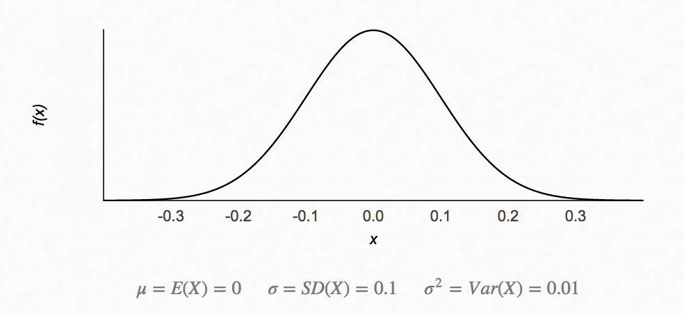
We can sample data using the PDF above. We use the following notation for sample data using a gaussian distribution with mean \(\mu\) and standard deviation \(\sigma\).

In the example above, mean: \(\mu=0\), standard deviation: \(\sigma=0.1\):

In many real world examples, the data sample distribution follows a gaussian distribution.

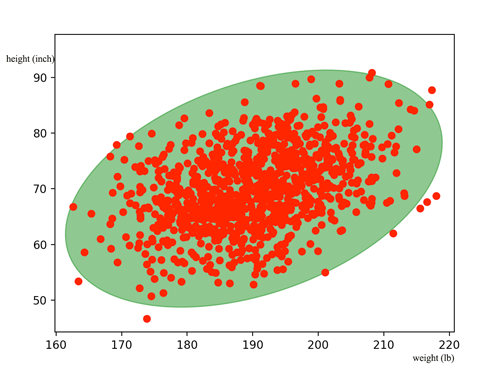
Now, we generalize it with multiple variables. For example, we want to model the relationship between the body height and the body weight for San Francisco residents. We collect the information from 1000 adult residents and plot the data below with each red dot represents 1 person:

We can plot the corresponding probability density function

in 3D:

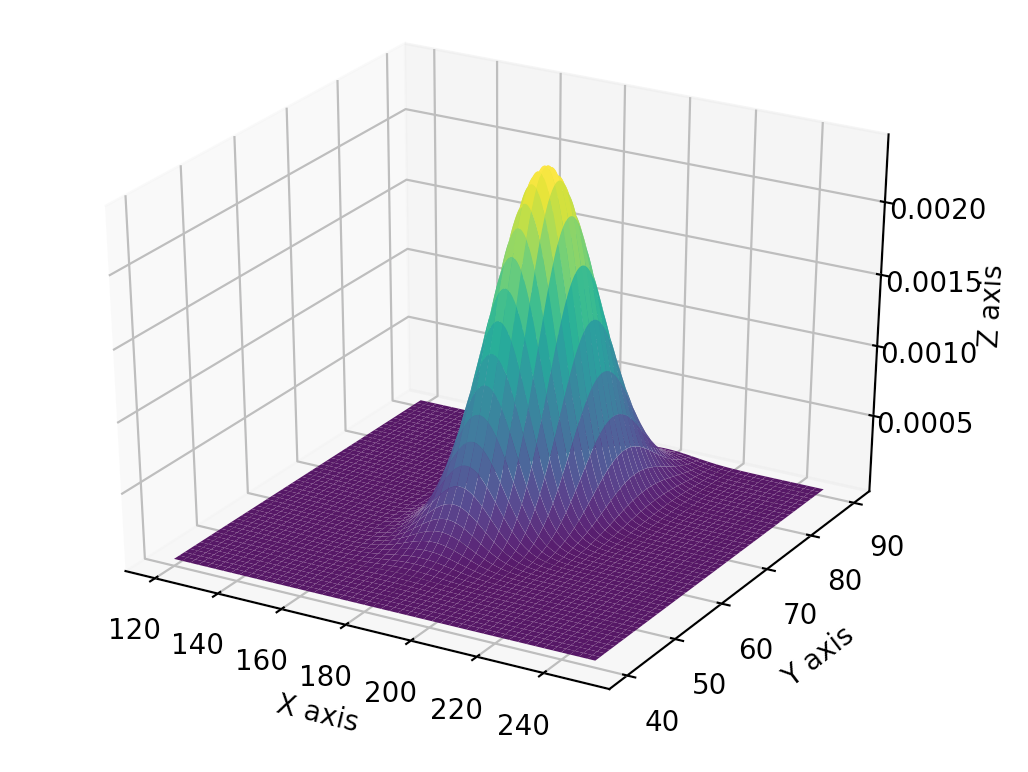
We can model usch probability density function using a gaussian distribution function.

The PDF with p variables is:

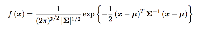
with covariance matrix \(\sum\):

The notation for sampling x is:

Let’s go back to our weight and height example to illustrate it.

From the data, we comput the mean weight is 190 lb and mean height is 70 inches:

For the covariance matrix \(\sum\), here, we illustrate how to compute one of the element \(E_{21}\)

which \(E\) is the expected value. Let say we have only 2 datapoints (200 lb, 80 inches) and (180 lb, 60 inches)

After computing all 1000 data, here is the value of \(\sum\):

\(E_{21}\) measures the co-relationship between variables \(x_2\) and \(x_1\). Positive values means both are positively related. With not surprise, \(E_{21}\) is positive because weight increases with height. If two variables are independent of each other, it should be 0 like:

and we will simplify the gaussian distribution notation here as: \(x \sim \mathcal{N}{\left( \begin{pmatrix} 190 \\ 70 \end{pmatrix} , \begin{pmatrix} 100 \\ 50 \\ \end{pmatrix} \right)}\)

Autoencoders

In an autoencoders, we use a deep network to map the input image (for example 256x256 pixels = 256x256 = 65536 dimension) to a lower dimension latent variables (latent vector say 100-D vector: \((x_1, x_2, \cdots x_{100})\)). We use another deep network to decode the latent variables to restore the image. We train both encoder and decoder network to minimize the difference between the original image and the decoded image. By forcing the image to a lower dimension, we hope the network learns to encode the image by extracting core features.

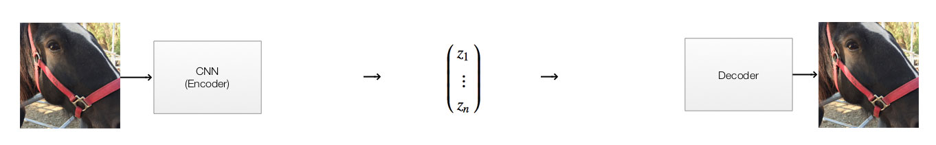
For example, we enter a 256x256 image to the encoder, we use a CNN to encode the image to 20-D latent variables \((x_1, x_1, ... x_{20}) = (0.1, 0, ..., -0.05)\). We use another network to decode the latent variables into a 256x256 image. We use backpropagation with cost function comparing the decoded and input image to train both encoding and decoding network.

Variational Autoencoders (VAEs)

For VAEs, we replace the middle part with a stochastic model using a gaussian distribution. Let’s get into an example to demonstrate the flow:

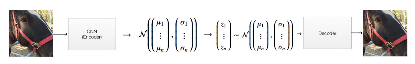
For a variation autoencoder, we replace the middle part with 2 separate steps. VAE does not generate the latent vector directly. It generates 100 Gaussian distributions each represented by a mean \((\mu_i)\) and a standard deviation \((\sigma_i)\). Then it samples a latent vector, say (0.1, 0.03, …, -0.01), from these distributions. For example, if element \(x_i\) of the latent vector has \(\mu_i=0.1\) and \(\sigma_i=0.5\). We randomly select \(x_i\) with probability based on this Gaussian distribution:

Say, the encoder generates \(\mu=(0, -0.01, ..., 0.2)\) and \(\sigma=(0.05, 0.01, ..., 0.02)\)

We can sample a value from this distribution:

with the latent variables as (say) :

The autoencoder in the previous section is very hard to train with not much guarantee that the network is generalize enough to make good predictions.(We say the network simply memorize the training data.) In VAEs, we add a constrain to make sure:

1. The latent variable are relative independent of each other, i.e. the 20 variables are relatively independent of each other (not co-related). This maximizes what a 20-D latent vectors can represent.
2. Latent variables \(z\) which are similar in values should generate similar looking images. This is a good indication that the network is not trying to memorize individual image.

To achieve this, we want the gaussian distribution model generated by the encoder to be as close to a normal gaussian distribution function. We penalize the cost function if the gaussian function is deviate from a normal distribution. This is very similar to the L2 regularization in a fully connected network in avoiding overfitting.

In a normal gaussian distribution, the covariance \(E_{ij}\) is 0 for \(i \neq j\). That is the latent variables are independent of each other. If the distribution is normalize, the distance between different \(z\) will be a good measure of its similarity. With sampling and the gaussian distribution, we encourage the network to have similar value of \(z\) for similar images.

Encoder

Here we have a CNN network with 2 convolution layers using leaky ReLU follow by one fully connected layer to generate 20 \(\mu\) and another fully connected layer for 20 \(\sigma\).

def recognition(self, input_images):
     with tf.variable_scope("recognition"):
         h1 = lrelu(conv2d(input_images, 1, 16, "d_h1"))   # Shape: (?, 28, 28, 1) -> (?, 14, 14, 16)
         h2 = lrelu(conv2d(h1, 16, 32, "d_h2"))            # (?, 7, 7, 32)
         h2_flat = tf.reshape(h2, [self.batchsize, 7 * 7 * 32])  # (100, 1568)

         w_mean = linear(h2_flat, self.n_z, "w_mean")      # (100, 20)
         w_stddev = linear(h2_flat, self.n_z, "w_stddev")  # (100, 20)

     return w_mean, w_stddev

Decoder

The decoder feeds the 20 latent variables to a fully connected layer followed with 2 transpose convolution layer with ReLU. The output is then feed into a sigmoid layer to generate the image.

def generation(self, z):
    with tf.variable_scope("generation"):
        z_develop = linear(z, 7 * 7 * 32, scope='z_matrix')  # (100, 20) -> (100, 1568)
        z_matrix = tf.nn.relu(tf.reshape(z_develop, [self.batchsize, 7, 7, 32]))  # (100, 7, 7, 32)
        h1 = tf.nn.relu(conv_transpose(z_matrix, [self.batchsize, 14, 14, 16], name="g_h1"))  # (100, 14, 14, 16)
        h2 = conv_transpose(h1, [self.batchsize, 28, 28, 1], name="g_h2")  # (100, 14, 14, 16)
        out = tf.nn.sigmoid(h2)  # (100, 28, 28, 1)

    return out     

Building the VAE

We use the encoder to encode the input image. Use sampling to generate \(z\) from the mean and variance of the gaussian distribution and then decode it.

# Encode the image
z_mean, z_stddev = self.recognition(image_matrix)
		
# Sampling z
samples = tf.random_normal([self.batchsize, self.n_z], 0, 1, dtype=tf.float32)
guessed_z = z_mean + (z_stddev * samples)

# Decode the image
self.generated_images = self.generation(guessed_z)
generated_flat = tf.reshape(self.generated_images, [self.batchsize, 28 * 28])

Cost function & training

We define a generation loss which measure the difference between the original and the decoded message using the mean square error. The latent loss measure the difference between gaussian function of the image from a normal distribution using KL-Divergence.

self.generation_loss = -tf.reduce_sum(
    self.images * tf.log(1e-8 + generated_flat) + (1 - self.images) * tf.log(1e-8 + 1 - generated_flat), 1)

self.latent_loss = 0.5 * tf.reduce_sum(
    tf.square(z_mean) + tf.square(z_stddev) - tf.log(tf.square(z_stddev)) - 1, 1)

self.cost = tf.reduce_mean(self.generation_loss + self.latent_loss)

We use the adam optimizer to train both networks.

self.optimizer = tf.train.AdamOptimizer(0.001).minimize(self.cost)

Cost function in detail

In VAE, we model the data distribution \(p(x)\) with an encoder \(q_𝜙(z \vert x)\) , a decoder \(p_𝜃(x \vert z)\) and a latent variable \(p(z)\) using the objective function:

To draw this conclusion, we start with the KL divergence which measures the difference of 2 distributions. By definition, KL divergence is defined as:

Apply it with:

Let \(q_𝜙 (z \vert x)\) be the distribution of \(z\) predicted by the encoder. Our objective is to minimize the KL divergence betwee the decoder \(q_𝜙 (z \vert x)\) and the ground truth distribution \(p(z \vert x)\). We want the distribution approximated by the deep network has little divergence from the true distribution. i.e. we want to optimize \(𝜙\) with the smallest KL divergence.

Apply:

Define the term ELBO (Evidence lower bound) as:

We call ELBO the evidence lower bound because:

Here, we define our VAE objective function

\[\log p(x) - D_{KL} [ q_𝜙 (z \vert x) \Vert p(z \vert x) ] = \mathbb{E}_q [ \log p (x \vert z)] - D_{KL} [q_𝜙 (z \vert x) \Vert p(z)]\]

Instead of the distribution \(p(x)\), we can model the data \(x\) with \(\log p(x)\). With the error term, \(D_{KL} [ q_𝜙 (z \vert x) \Vert p(z \vert x) ]\), we can establish a lower bound \(ELBO\) for \(\log p(x)\). In the VAE objective function, maximize our model probability \(\log p(x)\) is the same as maximize \(\log p (x \vert z)]\) while minimize the divergence of \(D_{KL} [q_𝜙 (z \vert x) \Vert p(z)]\).

Maximizing \(\log p (x \vert z)\) can be done by building a decoder network and maximize its likelihood. So with an encoder \(q_𝜙(z \vert x)\) , a decoder \(p_𝜃(x \vert z)\), our objective become optimizing:

We can apply a constrain to \(p(z)\) such that we can evaluate \(D_{KL} [ q_\phi (z \vert x) \Vert p(z) ]\) easily. In AVE, we use \(p(z) = \mathcal{N} (0, 1)\). For optimal solution, we want \(q_\phi (z \vert x)\) to be as close as \(\mathcal{N} (0, 1)\).

In VAE, we model \(q_\phi (z \vert x)\) as \(\mathcal{N} (\mu, \Sigma)\), the KL-divergence can be computed as:

KL-divergence of 2 Gaussian distributions

Here is an exercise in computing the KL divergence of 2 simple gaussian distributions:

Result

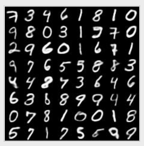
The full source code for the VAE is located here. Here is the digits created by a VAE.

Credits

Part of the source code for GAN & Variational Autoencoders is originated from https://github.com/kvfrans/generative-adversial and https://github.com/carpedm20/DCGAN-tensorflow.