“Class visualization, style transfer and DeepDream”
Discriminative models
In a discriminative model, we draw conclusion on something we observe. For example, we train a CNN discriminative model to classify a picture.
\[y = f(image)\]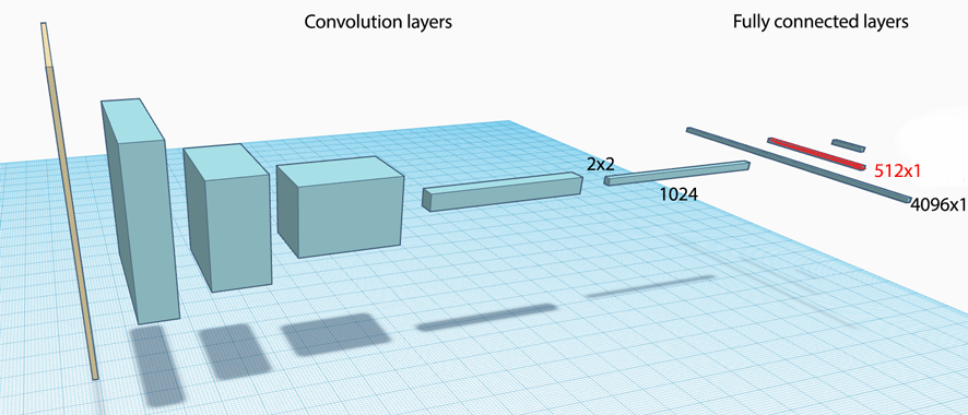
Class visualization
Often, we want to visualize what features a network tries to learn in the classification process. First, we train a classification CNN model. Then we genearte a random image and feed forward to the network. Instead of backpropagate the gradient to train \(W\), we backpropagate the gradient to make \(image\) to look like the target class. i.e., use backpropagation to change the \(image\) to increase the score of the target class. In order to do so, we change \(\frac{\partial J}{\partial score_i}\) manually to:
\[\frac{\partial J}{\partial score_i}= \left\{ \begin{array}{lr} 1,& i=target \\ 0,& i \neq target \end{array} \right\}\], and reiterate the feed forward and backward many times. Here is the skeleton code to generate an image from a pre-trained CNN model for the target class target_y.
def class_visualization(target_y, model, learning_rate, l2_reg, num_iterations):

    # Generate a random image
    X = np.random.randn(1, 3, 64, 64)
    for t in xrange(num_iterations):
        dX = None
        scores, cache = model.forward(X, mode='test')

        # Artifically set the dscores for our target to 1, otherwise 0.
        dscores = np.zeros_like(scores)
        dscores[0, target_y] = 1.0

        # Backpropagate
        dX, grads = model.backward(dscores, cache)
        dX -= 2 * l2_reg * X

        # Change the image with the gradient descent.
        X += learning_rate * dX
    return X
To make it works better, we add clipping, jittering and blurring:
def class_visualization(target_y, model, learning_rate, l2_reg, num_iterations, blur_every, max_jitter):
    X = np.random.randn(1, 3, 64, 64)
    for t in xrange(num_iterations):
        # Add the jitter
        ox, oy = np.random.randint(-max_jitter, max_jitter + 1, 2)
        X = np.roll(np.roll(X, ox, -1), oy, -2)

        dX = None
        scores, cache = model.forward(X, mode='test')

        dscores = np.zeros_like(scores)
        dscores[0, target_y] = 1.0
        dX, grads = model.backward(dscores, cache)
        dX -= 2 * l2_reg * X

        X += learning_rate * dX

        # Undo the jitter
        X = np.roll(np.roll(X, -ox, -1), -oy, -2)

        # As a regularizer, clip the image
        X = np.clip(X, -data['mean_image'], 255.0 - data['mean_image'])

        # As a regularizer, periodically blur the image
        if t % blur_every == 0:
            X = blur_image(X)
    return X
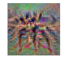
Here is our attempt to generate a spider image starting from random noises.
Artistic Style Transfer
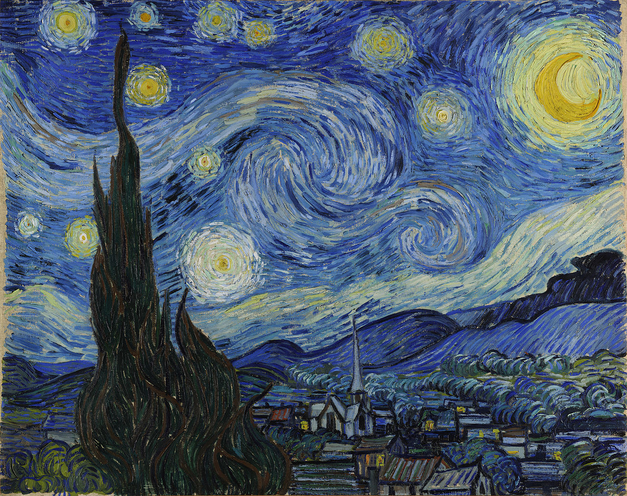
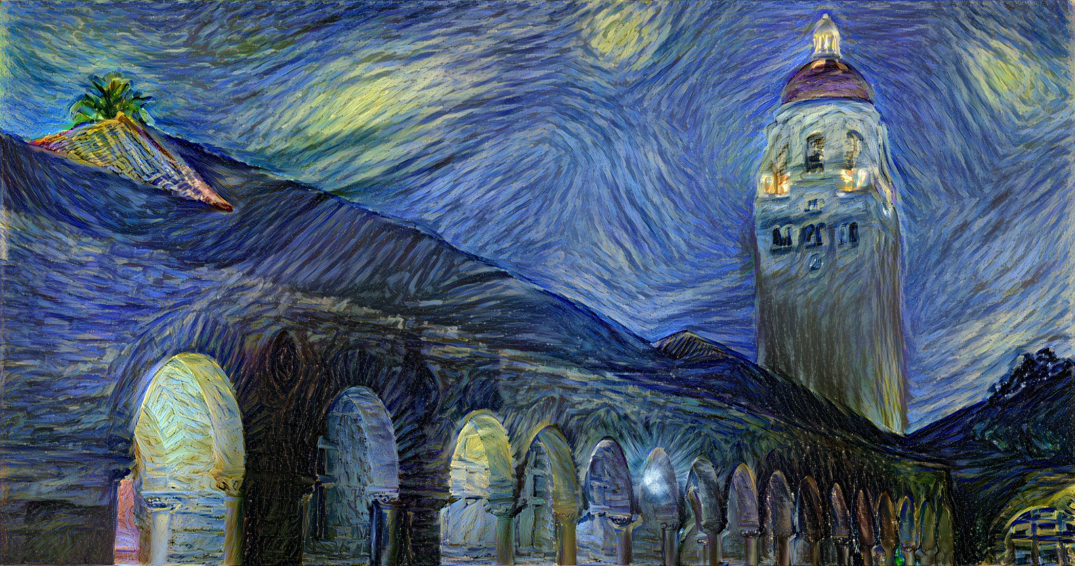
Artistic style transfer applies the style of one image to another. We start with a picture as our style image
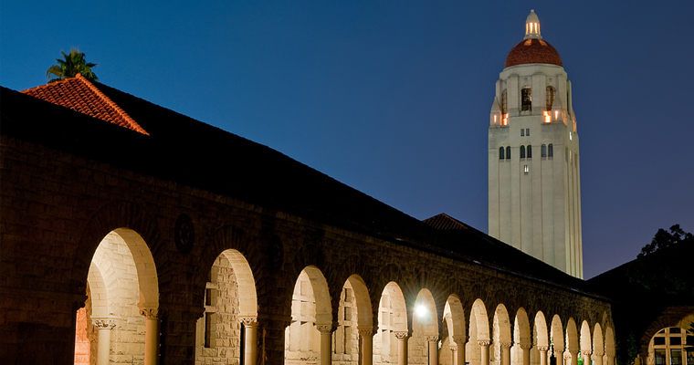
, and transfer the style to another content image
to create the result image.
We start with a random result image. The key idea of the style transfer is to extract the content features from the content image and the style features from the style image. Then we apply backpropagation to the result image with a cost function
- measuring the content difference between the content image and the result image, and
- the style difference between the style image and result image.
After many iterations, the result image will conform to an image with the content structure of the content image and the style of the style image.
Recall a CNN composes of many convolution layers follow with fully connected layers:
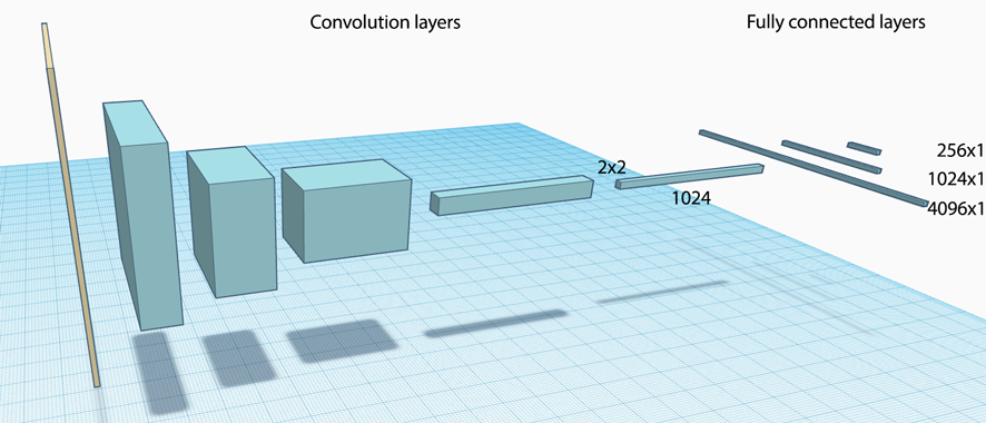
A VGG-19 network uses 19 layers to process images of size 224x224x3. It has 5 major convolution layers and 3 fully connected layers.
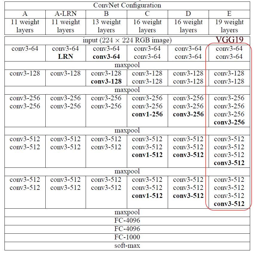
Here is the configuration within each major CNN convolution layer:
| Convolution/ReLU/pooling | Feature dimension | |
| CNN layer 1 | ‘conv1_1’ -> ‘relu1_1’ -> ‘conv1_2’ -> ‘relu1_2’ -> ‘pool1’ | 112x112x64 |
| CNN layer 2 | ‘conv2_1’ -> ‘relu2_1’ -> ‘conv2_2’ -> ‘relu2_2’ -> ‘pool2’ | 56x56x128 |
| CNN layer 3 | ‘conv3_1’ -> ‘relu3_1’ -> ‘conv3_2’ -> ‘relu3_2’ -> ‘conv3_3’ -> ‘relu3_3’ -> ‘conv3_4’ -> ‘relu3_4’ -> ‘pool3’ | 28x28x256 |
| CNN layer 4 | ‘conv4_1’ -> ‘relu4_1’ -> ‘conv4_2’ -> ‘relu4_2’ -> ‘conv4_3’ -> ‘relu4_3’ -> ‘conv4_4’ -> ‘relu4_4’ -> ‘pool4’ | 14x14x512 |
| CNN layer 5 | ‘conv5_1’ -> ‘relu5_1’ -> ‘conv5_2’ -> ‘relu5_2’ -> ‘conv5_3’ -> ‘relu5_3’ -> ‘conv5_4’ -> ‘relu5_4’ | 7x7x512 |
The following is the visualization of features that each layer try to capture:
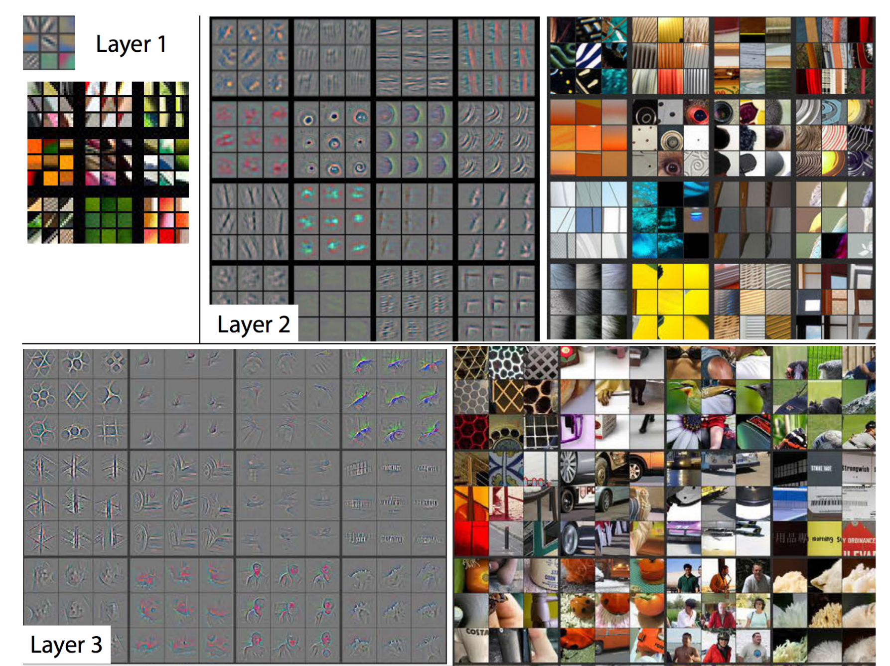
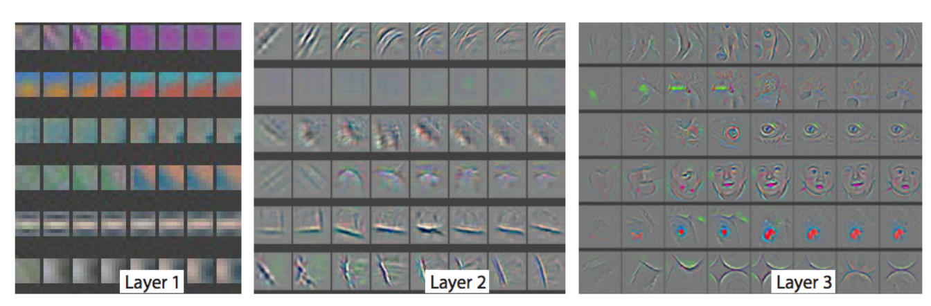
In the first couple layers, CNN try to capture smaller scale feature like edges, strokes as well as color. Only larger scale structure is shown in layer 3 or later.
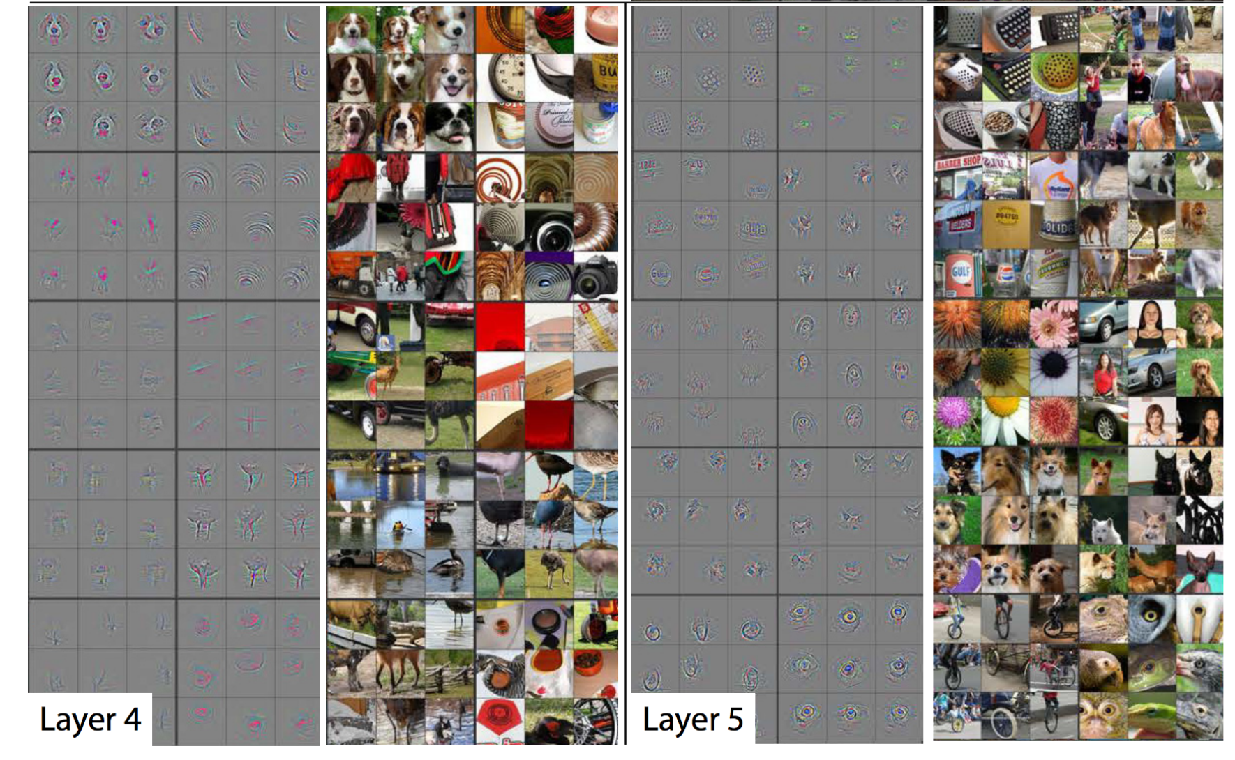
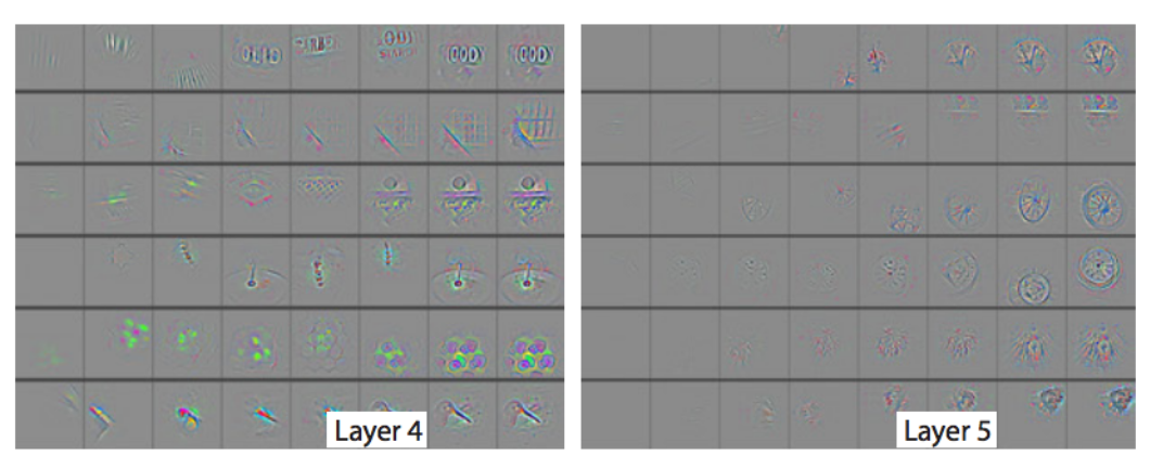
In layer 4 and 5, we can identify the content of the image much easily. Early layers capture edges, strokes and color which characterize an image style while later layers capture structure (content). From this observation, we use early layers to capture style and the later layers for content. In our code example, we use layers ‘relu1_1’, ‘relu2_1’, ‘relu3_1’, ‘relu4_1’, ‘relu5_1’ to extract style while using ‘relu4_2’ and ‘relu5_2’ to capture content.
Content features
We first load the parameters of a pre-trained VGG-19 network.
vgg_weights, vgg_mean_pixel = vgg.load_net(network) # Load the VGG-19 parameters
We create a placeholder for the image. Load the weights (parameters) for the VGG-19 model with vgg.net_preloaded. Create an operation to subtract the image from the mean pixel. The we create operators to compute the content feature from layer “relu4_2” and “relu5_2” using the VGG-19 model.
g = tf.Graph()
with g.as_default(), g.device('/cpu:0'), tf.Session() as sess:
    image = tf.placeholder('float', shape=shape)

    # Load VGG-19 model {'conv1_1': Tensor..., relu1_1: Tensor...}
    net = vgg.net_preloaded(vgg_weights, image, pooling)

    # (1, 533, 400, 3) subtract with the mean pixel
    content_pre = np.array([vgg.preprocess(content, vgg_mean_pixel)])

    for layer in CONTENT_LAYERS:     # (relu4_2, relu5_2)
        # Find the feature values for (relu4_2, relu5_2)
        content_features[layer] = net[layer].eval(feed_dict={image: content_pre})
Style features
Similarly we extract the style features of the style images in layer ‘relu1_1’, ‘relu2_1’, ‘relu3_1’, ‘relu4_1’ and ‘relu5_1’. Then we convert the features to a Gram matrix which will be stored as the style features. A Gram matrix is defined as:
\[G(x_1, x_2, \dots, x_n) = \begin{pmatrix} \lt x_1, x_1 \gt & \lt x_1, x_2 \gt & \dots & \lt x_1, x_n \gt \\ \lt x_2, x_1 \gt & \lt x_2, x_2 \gt & \dots & \lt x_2, x_n \gt \\ \vdots & \vdots & \ddots & \vdots \\ \lt x_n, x_1 \gt & \lt x_n, x_2 \gt & \dots & \lt x_n, x_n \gt \\ \end{pmatrix} %]]>\]which \(\lt x_i, x_j \gt\) is the inner product of 2 vectors. Dot product measures the similarity of 2 features: it reaches the maximum if they are the same or zero if they are not related. This Gram matrix measures the relationships between features. For example, how certain strokes may related with each other or with some color. We compute the Gram matrices for the style image and the result image. We want both Gram matrices to be as close as possible.
g = tf.Graph()
with g.as_default(), g.device('/cpu:0'), tf.Session() as sess:
    # Set up image placeholder and the VGG-19 model
    # (1, 316, 400, 3)
    image = tf.placeholder('float', shape=style_shapes[i])
    net = vgg.net_preloaded(vgg_weights, image, pooling)
    style_pre = np.array([vgg.preprocess(styles[i], vgg_mean_pixel)])
    for layer in STYLE_LAYERS:  # ('relu1_1', 'relu2_1', 'relu3_1', 'relu4_1', 'relu5_1')
        # For relu1_1 layer, features: (1, 316, 400, 64)
        features = net[layer].eval(feed_dict={image: style_pre})
        features = np.reshape(features, (-1, features.shape[3]))      # (126400, 64)
        gram = np.matmul(features.T, features) / features.size        # (64, 64) Gram matrix
        style_features[layer] = gram
Result image
We randomize an initial image with Gaussian Distribution with the same \(\sigma\) as the content image.
# Generate a random image with SD the same as the content image.
noise = np.random.normal(size=shape, scale=np.std(content) * 0.1)
initial = tf.random_normal(shape) * 0.256
We build another VGG-19 model for the result image.
with tf.Graph().as_default():
    initial = np.array([vgg.preprocess(initial, vgg_mean_pixel)])
    initial = initial.astype('float32')

    image = tf.Variable(initial)
    net = vgg.net_preloaded(vgg_weights, image, pooling)
Content loss
We compute the content loss which is the mean square error (MSE) of the features in the result image and the features in the content image.
tf.nn.l2_loss(
   net[content_layer] - content_features[content_layer]
)
We add all the content loss for the layer ‘relu4_2’ and ‘relu5_2’. For each layer, we can use a different weight that is configurable by the user.
# content loss
content_layers_weights = {}
content_layers_weights['relu4_2'] = content_weight_blend
content_layers_weights['relu5_2'] = 1.0 - content_weight_blend

content_loss = 0
content_losses = []
for content_layer in CONTENT_LAYERS:       # {'relu4_2', 'relu5_2'}
   # Use MSE as content losses
   content_losses.append(content_layers_weights[content_layer] *
	       content_weight *
	       (2 * tf.nn.l2_loss(net[content_layer] - content_features[content_layer])
				  / content_features[content_layer].size))
     content_loss += reduce(tf.add, content_losses)
Style loss
We compute the Gram matrix of the result image. The style loss is define as the MSE of the difference between the Gram matrix of the result image and the style image.
tf.nn.l2_loss(gram - style_gram)
We add all the L2 loss using the Gram matrix for the result image and the style image. For each layer, we can use a different weight that is configurable by the user.
# style loss
style_loss = 0
style_losses = []
for style_layer in STYLE_LAYERS: # (relu1_1, relu2_1, relu3_1, relu4_1, relu5_1)
    layer = net[style_layer]     # For relu1_1: (1, 533, 400, 64)
    _, height, width, number = map(lambda i: i.value, layer.get_shape())
    size = height * width * number
    feats = tf.reshape(layer, (-1, number))     # (213200, 64)

    # Gram matrix for the features in relu1_1 for the result image.
    gram = tf.matmul(tf.transpose(feats), feats) / size

    # Gram matrix for the style image
    style_gram = style_features[style_layer]

    # Style loss is the MSE for the difference of the 2 Gram matrix
    style_losses.append(style_layers_weights[style_layer]
          * 2 * tf.nn.l2_loss(gram - style_gram) / style_gram.size)
    style_loss += style_weight * style_blend_weights[i] * reduce(tf.add, style_losses)
Noise loss
We add a extra cost with the purpose of reducing noise in the image. We shift the image by one pixel in both vertical or horizontal direction. By comparing the original and the shifted image, we add a L2 cost which will penalize if the generated result images are noisy.
# Total variation denoising: Add cost to penalize neighboring pixel is very different.
# This help to reduce noise.
tv_y_size = _tensor_size(image[:,1:,:,:])
tv_x_size = _tensor_size(image[:,:,1:,:])
tv_loss = tv_weight * 2 * (
              (tf.nn.l2_loss(image[:,1:,:,:] - image[:,:shape[1]-1,:,:]) /
                    tv_y_size) +
              (tf.nn.l2_loss(image[:,:,1:,:] - image[:,:,:shape[2]-1,:]) /
                    tv_x_size))
# overall loss
loss = content_loss + style_loss + tv_loss
Now we train the network:
# optimizer setup
train_step = tf.train.AdamOptimizer(learning_rate, beta1, beta2, epsilon).minimize(loss)

# optimization
with tf.Session() as sess:
     sess.run(tf.global_variables_initializer())
     for i in range(iterations):
         train_step.run()
The full source code is in Github. The source code is originated from https://github.com/anishathalye/neural-style/.
Google DeepDream
Google DeepDream uses a CNN to find and enhance features within an image. It forward feed an image to a CNN network to extract features at a particular layer. It then start backpropagate from that particular later with gradient set to:
\[\frac{\partial J}{\partial layer} = activation_{layer}\]This exaggerate the features at the chosen layer of the network.
# Feed foward until it reaches "layer"
out, cache = model.forward(X, end=layer)

# Start backpropagation from "layer"
dX, grads = model.backward(out, cache)

X += learning_rate * dX
Here, we start with an image of a cat:
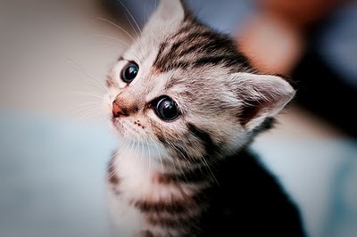
This is the image after many iterations:
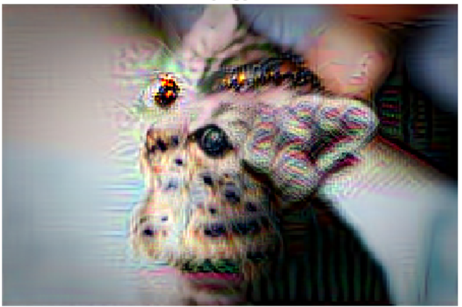
We turn around a CNN network to generate realistic images through backpropagation by exaggerate certain features.
Feature Inversion
Feature inversion is another technique using backpropagation to make a random image looks like another image. We select a particular layer and backpropagate the feature difference between the origina image and the content image. Abstraction increases as we move deeper into the network. The deeper we go, the more abstract on the result image.
out_feats, cache = model.forward(X, end=layer)
dout = 2 * (out_feats - target_feats)
dX, grads = model.backward(dout, cache)
dX += 2 * l2_reg * np.sum(X**2, axis=0)

X -= learning_rate * dX