“Fast R-CNN and Faster R-CNN”
I am retiring this page now.
-
If you are interested in Fast R-CNN, Faster R-CNN & FPN, we have better updated information at [medium.com/@jonathan_hui/what-do-we-learn-from-region-based-object-detectors-faster-r-cnn-r-fcn-fpn-7e354377a7c9].
-
If you are interested in single shot object detector like SSD and YOLO including YOLOv3, please visit [medium.com/@jonathan_hui/what-do-we-learn-from-single-shot-object-detectors-ssd-yolo-fpn-focal-loss-3888677c5f4d].
Object detection
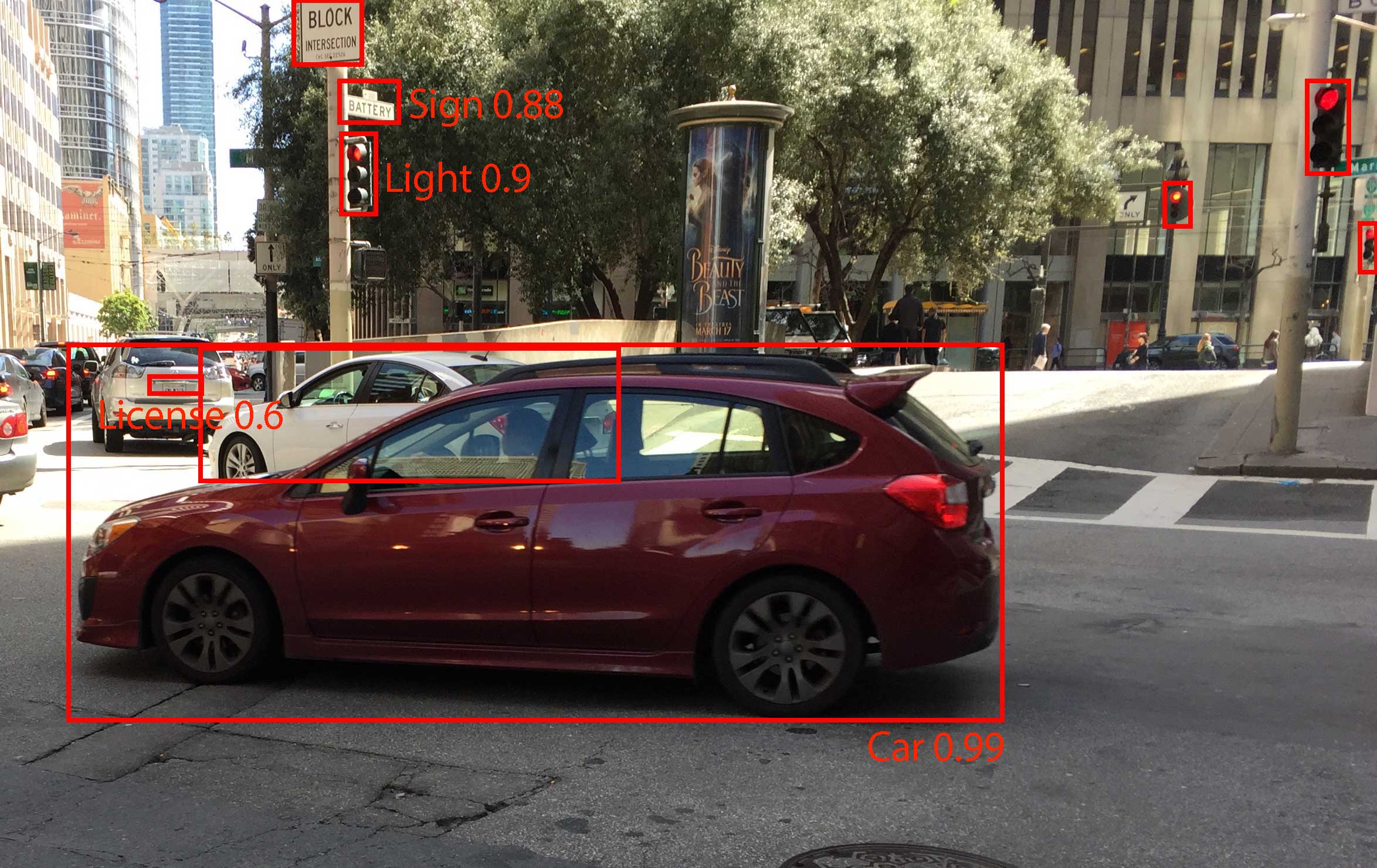
Detecting objects and their locations are critical for many Artificial Intelligence (AI) applications. For example, in autonomous driving, it is important to realize what objects are in front of us, as well as identifying traffic lights and road signs. The license plate reader in a police car alerts the authority of stolen cars by locating the license plates and applying visual recognition. The following picture illustrates some of the objects detected with the corresponding boundary box and estimated certainty. Object detection is about classifying objects and define a bounding box around them.
Regions with CNN features (R-CNN)
The information in R-CNN and the corresponding diagrams are based on the paper Rich feature hierarchies for accurate object detection and semantic segmentation, Ross Girshick et al.
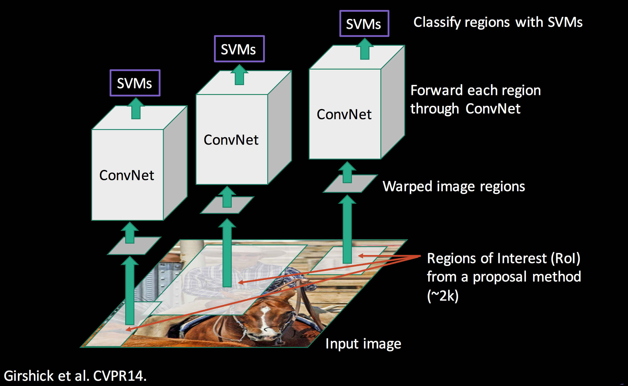
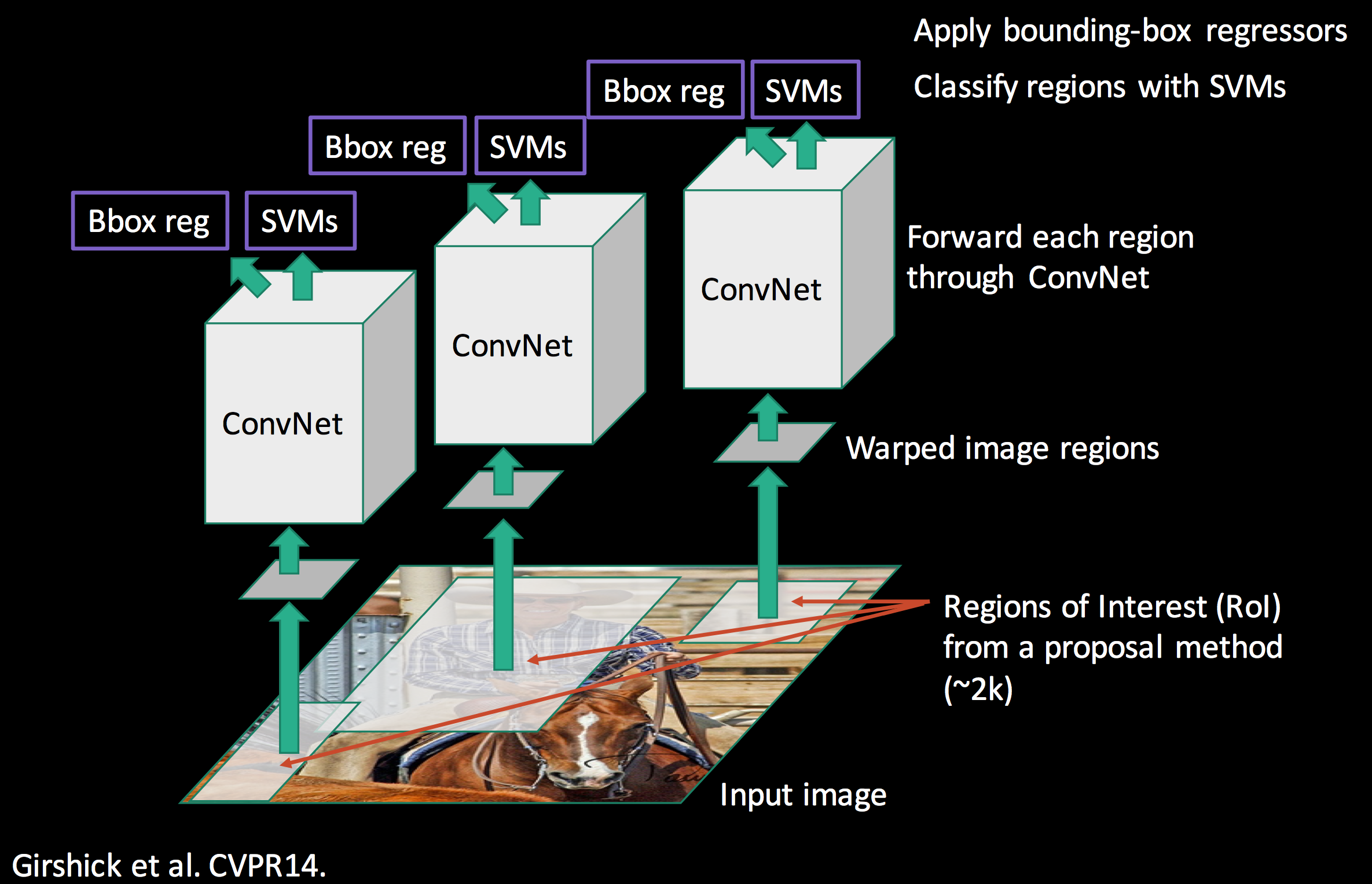
R-CNN overview
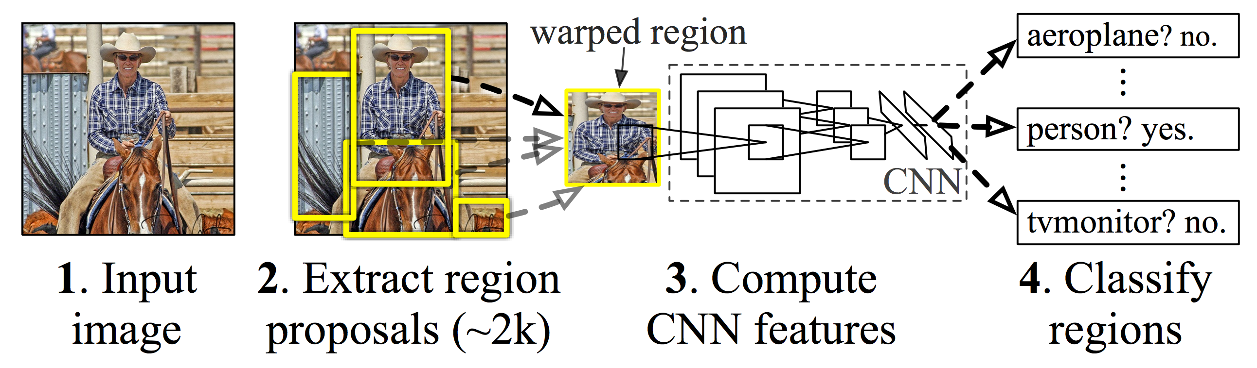
With an image, we:
- Extract region proposals: Use a region-extraction algorithm to propose about 2,000 objects’ boundaries.
- For each region proposal,
- Warp it to a size fitted for the CNN.
- Compute the CNN features.
- Classify what is the object in this region.
Use Selective search for region proposals
The information in selective search is based on the paper Segmentation as Selective Search for Object Recognition, van de Sande et al.
In selective search, we start with many tiny initial regions. We use a greedy algorithm to grow a region. First we locate two most similar regions and merge them together. Similarity \(S\) between region \(a\) and \(b\) is defined as:
\[S(a, b) = S_{texture}(a, b) + S_{size} (a, b).\]where \(S_{texture}(a, b)\) measures the visual similarity, and \(S_{size}\) prefers merging smaller regions together to avoid a single region from gobbling up all others one by one.
We continue merging regions until everything is combined together. In the first row, we show how we grow the regions, and the blue rectangles in the second rows show all possible region proposals we made during the merging. The green rectangle are the target objects that we want to detect.
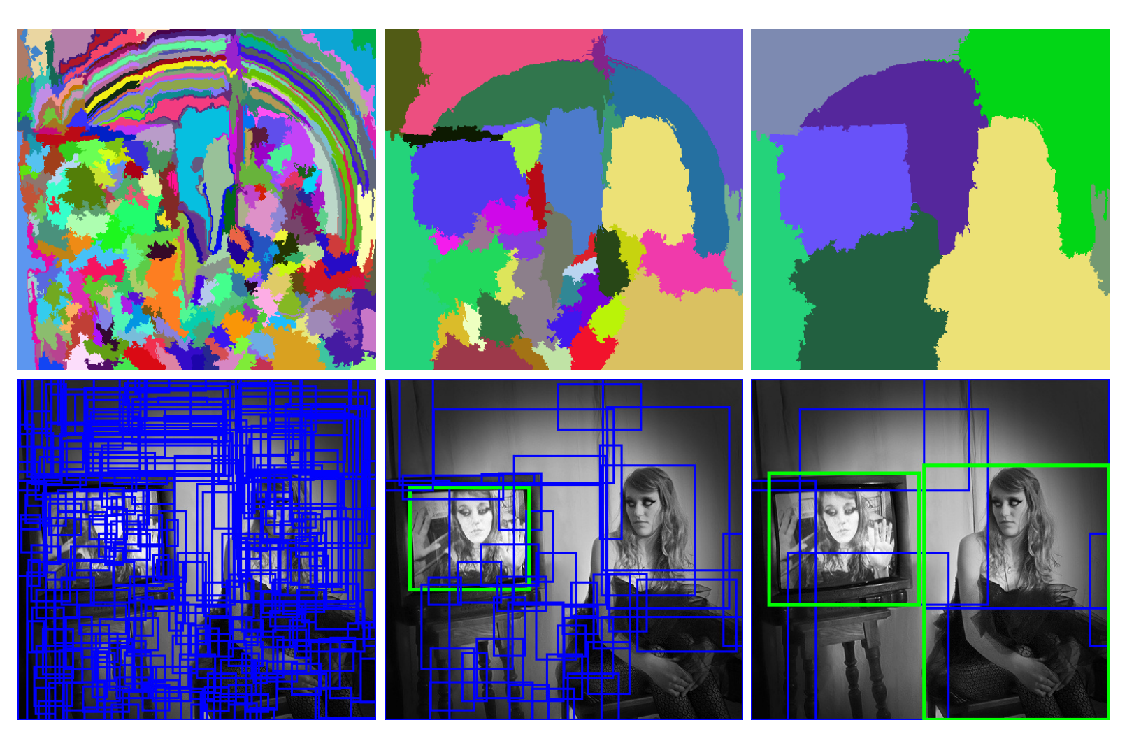
(Image source: van de Sande et al. ICCV’11)
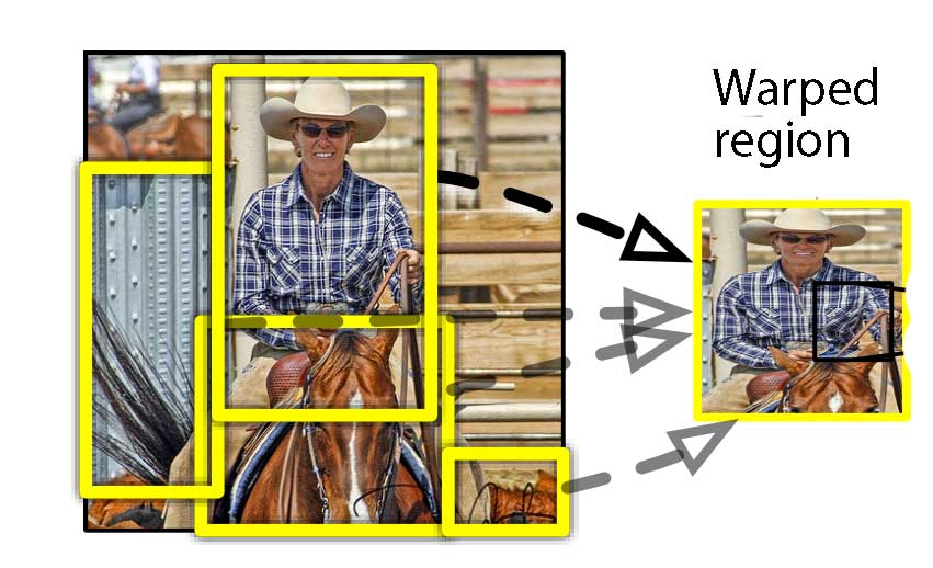
Warping
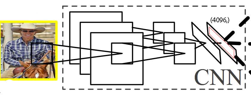
For every region proposal, we use a CNN to extract the features. Since a CNN takes a fixed-size image, we wrap a proposed region into a 227 x 227 RGB images.
Extracting features with a CNN
This will then process by a CNN to extract a 4096-dimensional feature:
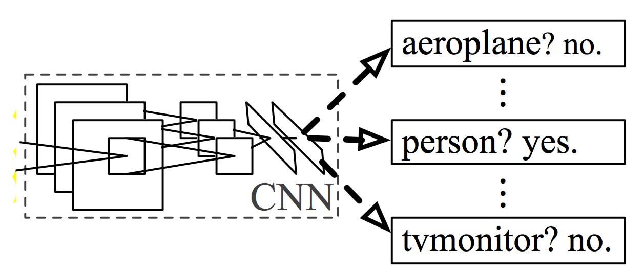
Classification
We then apply a SVM classifier to identify the object:
Putting it together
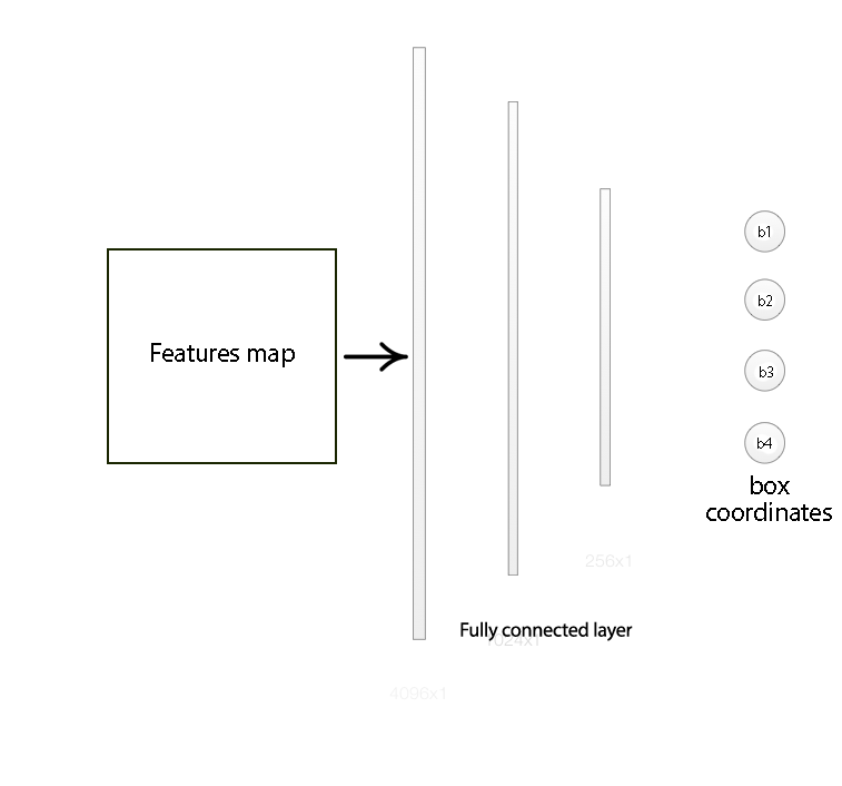
Bounding box regressor
The original boundary box proposal may need further refinement. We apply a regressor to calculate the final red box from the initial blue proposal region.
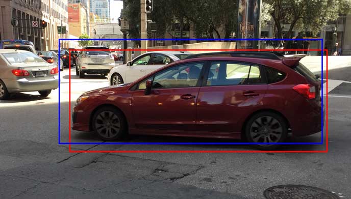
Here, the R-CNN classifies objects in a picture and produces the corresponding boundary box.
SPPnet & Fast R-CNN
The information and diagrams in this section come from “Spatial Pyramid Pooling in Deep Convolutional Networks for Visual Recognition”, Kaiming He et al for SPPnet and “Fast CNN”, Ross Girshick (ICCV’15) for Fast R-CNN
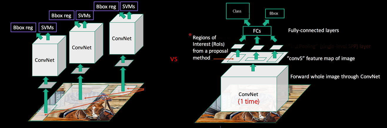
R-CNN is slow in training & inference. We have 2,000 proposals which each of them needed to be processed by a CNN to extract features, and therefore, R-CNN will repeat the ConvNet 2,000 times to extract features.
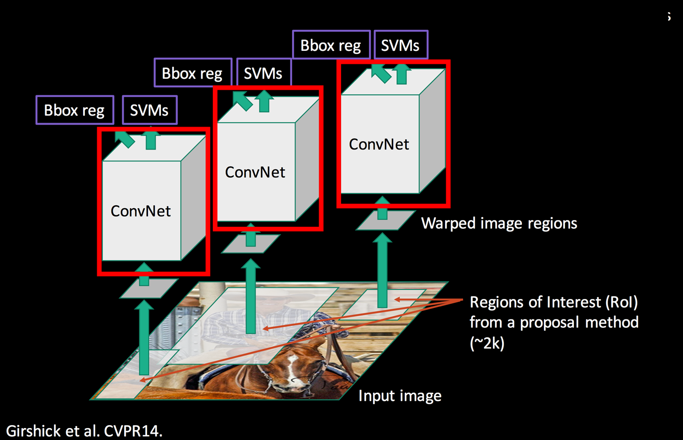
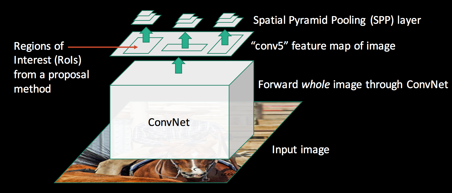
Hence, instead of converting 2,000 regions into the corresponding features maps, we convert the whole image once.
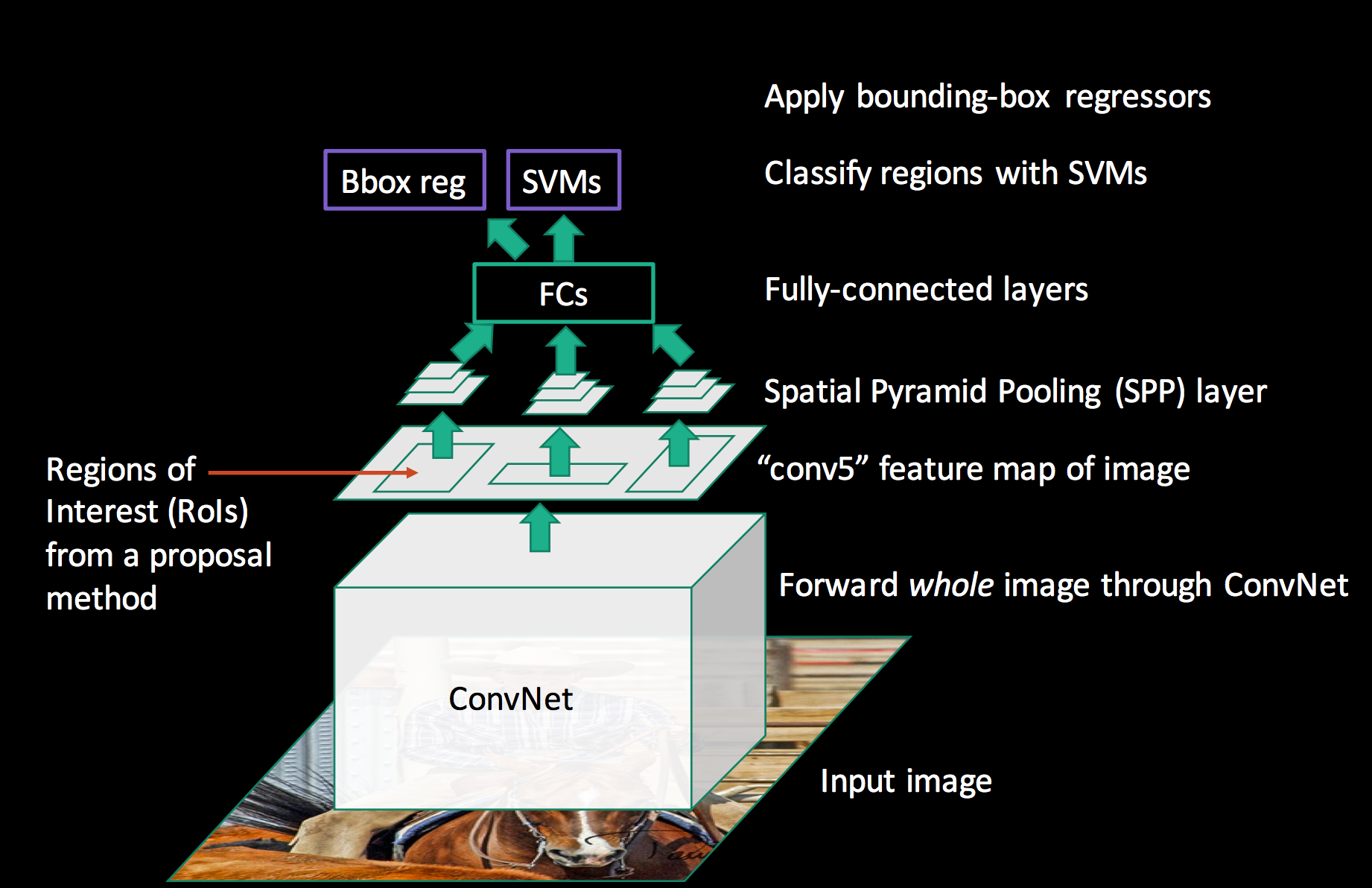
SPPnet
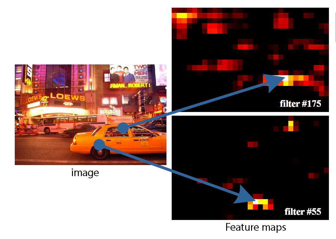
Here is the visualization of the features maps in a CNN.
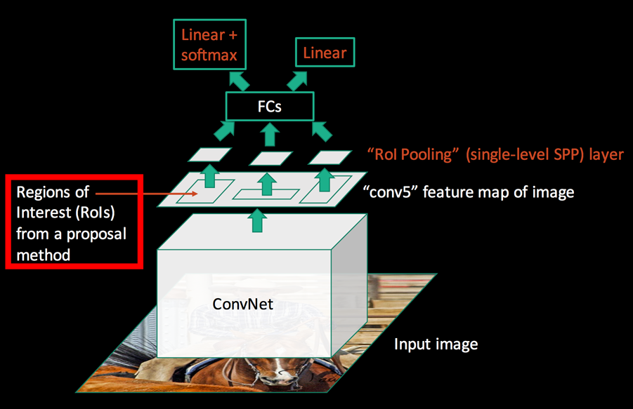
SPPnet uses a regional proposal method to generate region of interests (RoIs). The blue rectangular below shows one possible region of interest:
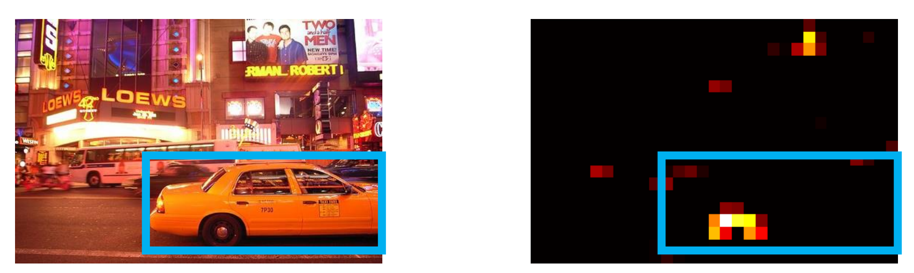
Both papers do not restrict themselves to any region proposal methods.
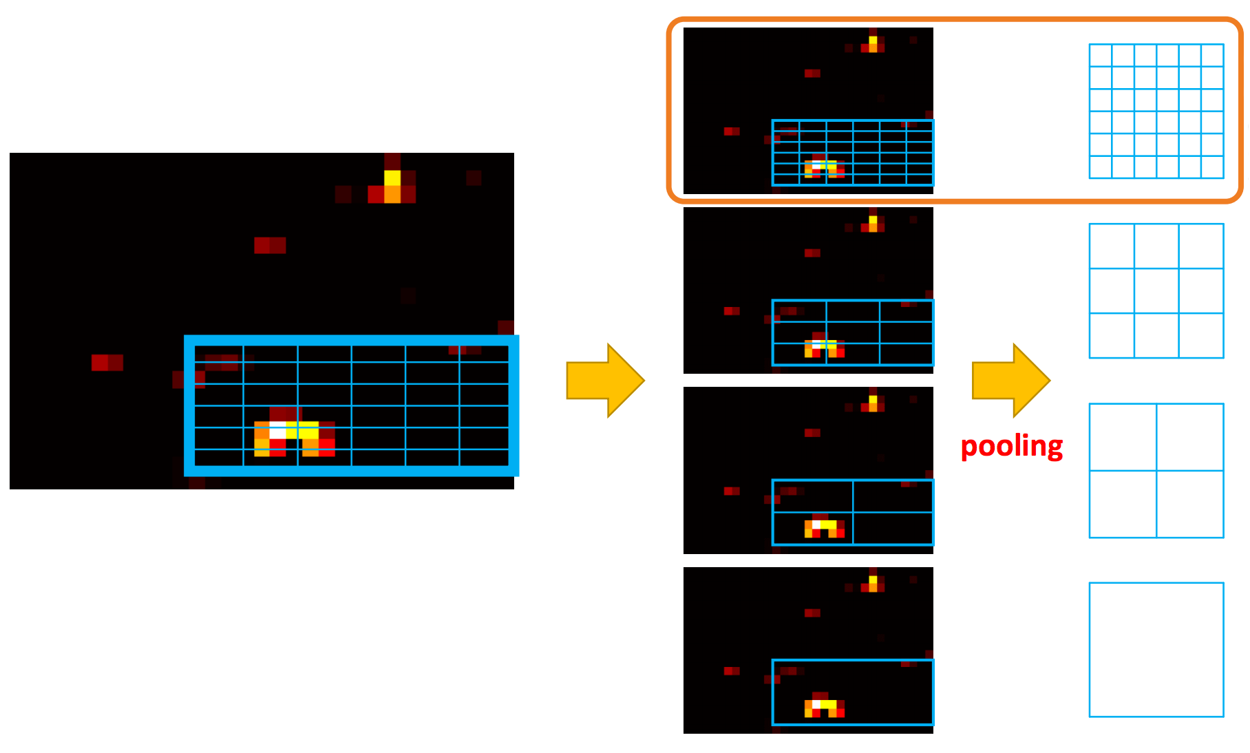
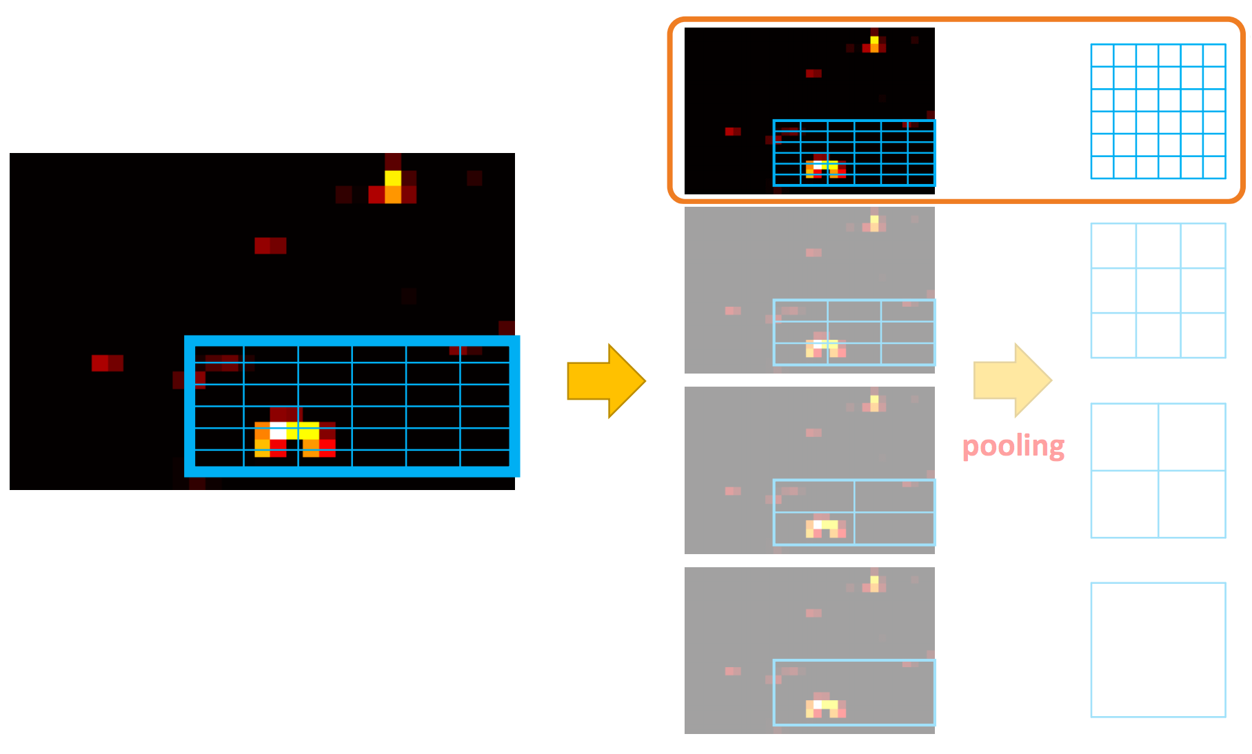
Here we warp region of interests (RoIs) into spatial pyramid pooling (SPP) layers.
Each spatial pyramid layer is in a different scale, and we use maximum pooling to warp the original RoI to the target map on the right.
We pass it to a fully-connected network, and use a SVM for classification and a linear regressor for the bounding box.
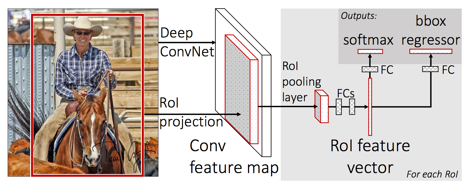
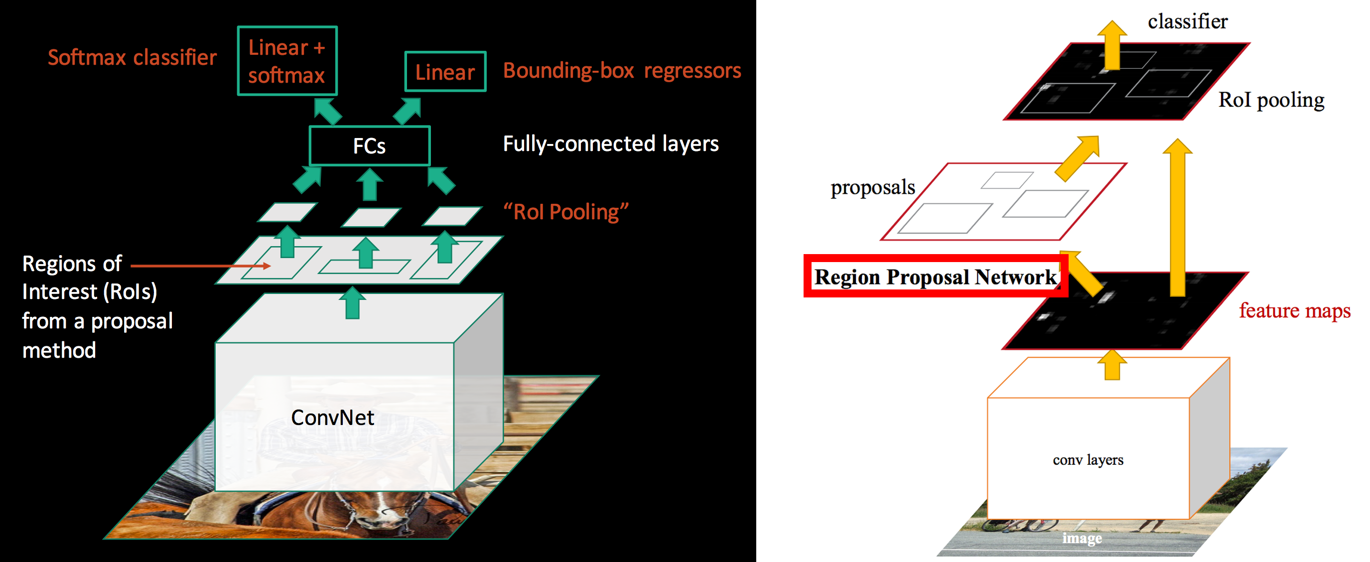
Fast R-CNN
Instead of generating a pyramid of layers, Fast R-CNN warps ROIs into one single layer using the RoI pooling.
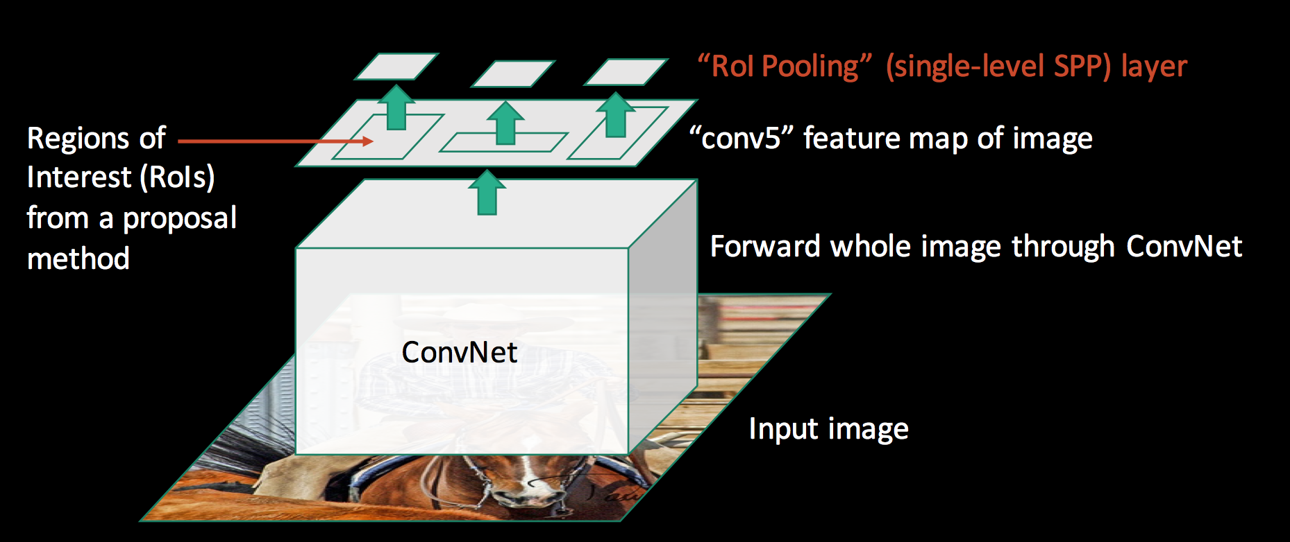
The RoI pooling layer uses max pooling to convert the features in a region of interest into a small feature map of H × W. Both H & W (e.g., 7 × 7) are tunable hyper-parameters.
You can consider Fast R-CNN is a special case of SPPNet. Instead of multiple layers, Fast R-CNN only use one layer.
It is feed into a fully-connected network for classification using linear regression and softmax. The bounding box is further refined with a linear regression.
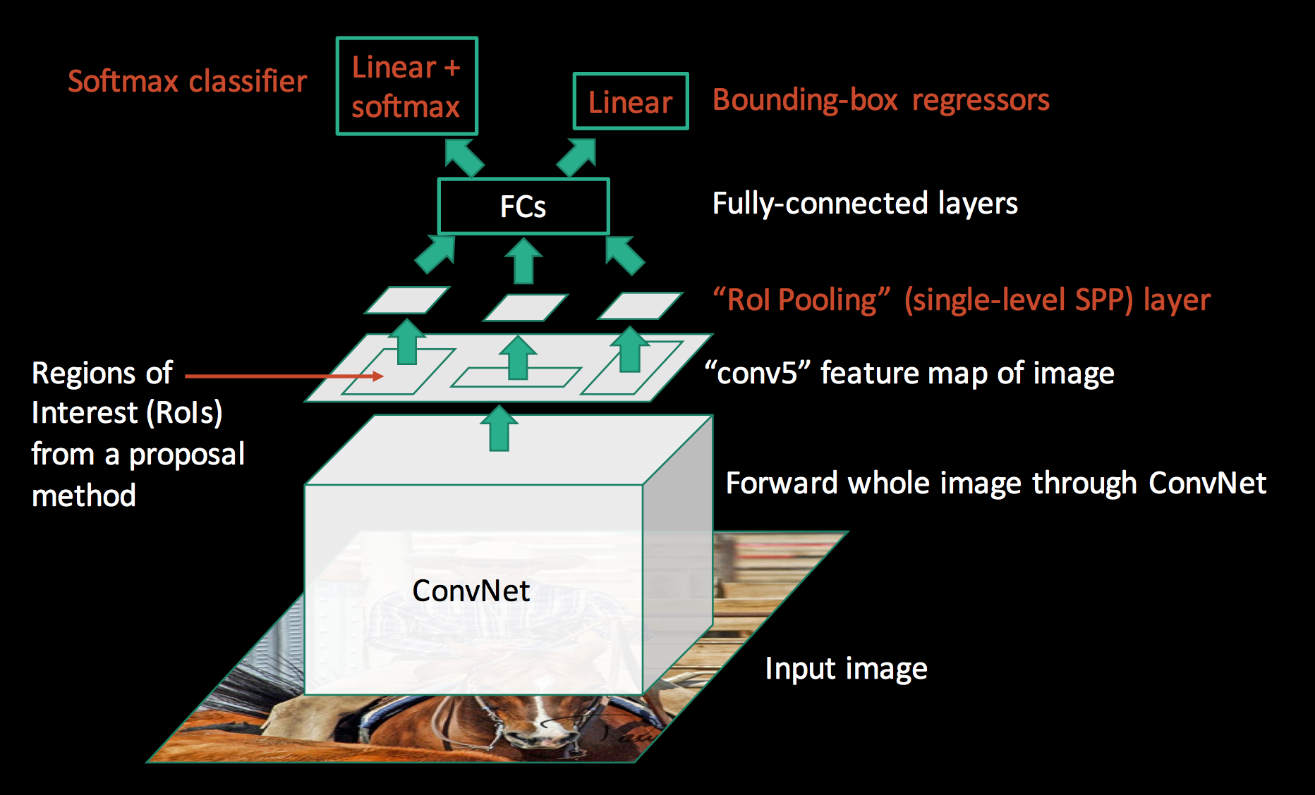
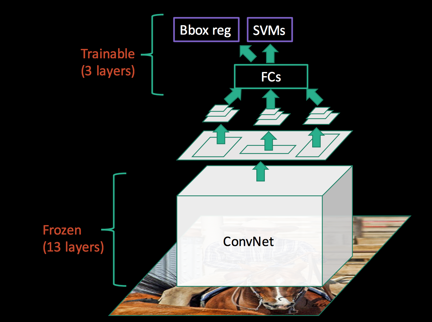
The key difference between SPPnet and Fast R-CNN is that SPPnet cannot update parameters below SPP layer during training:
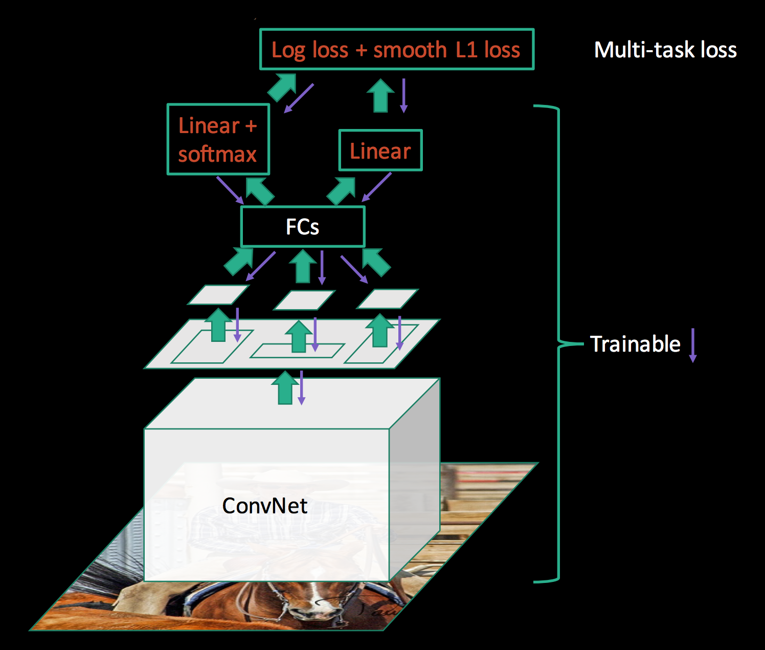
In Fast R-CNN, all parameters including the CNN can be trained together. All the parameters are trained together with a log loss function from the class classification and a L1 loss function from the boundary box prediction.
Faster R-CNN
The information and some diagrams in this section are based on the paper Faster R-CNN: Towards Real-Time Object Detection with Region Proposal Networks, Shaoqing Ren etc al
Both SPPnet and Fast R-CNN requires a region proposal method.
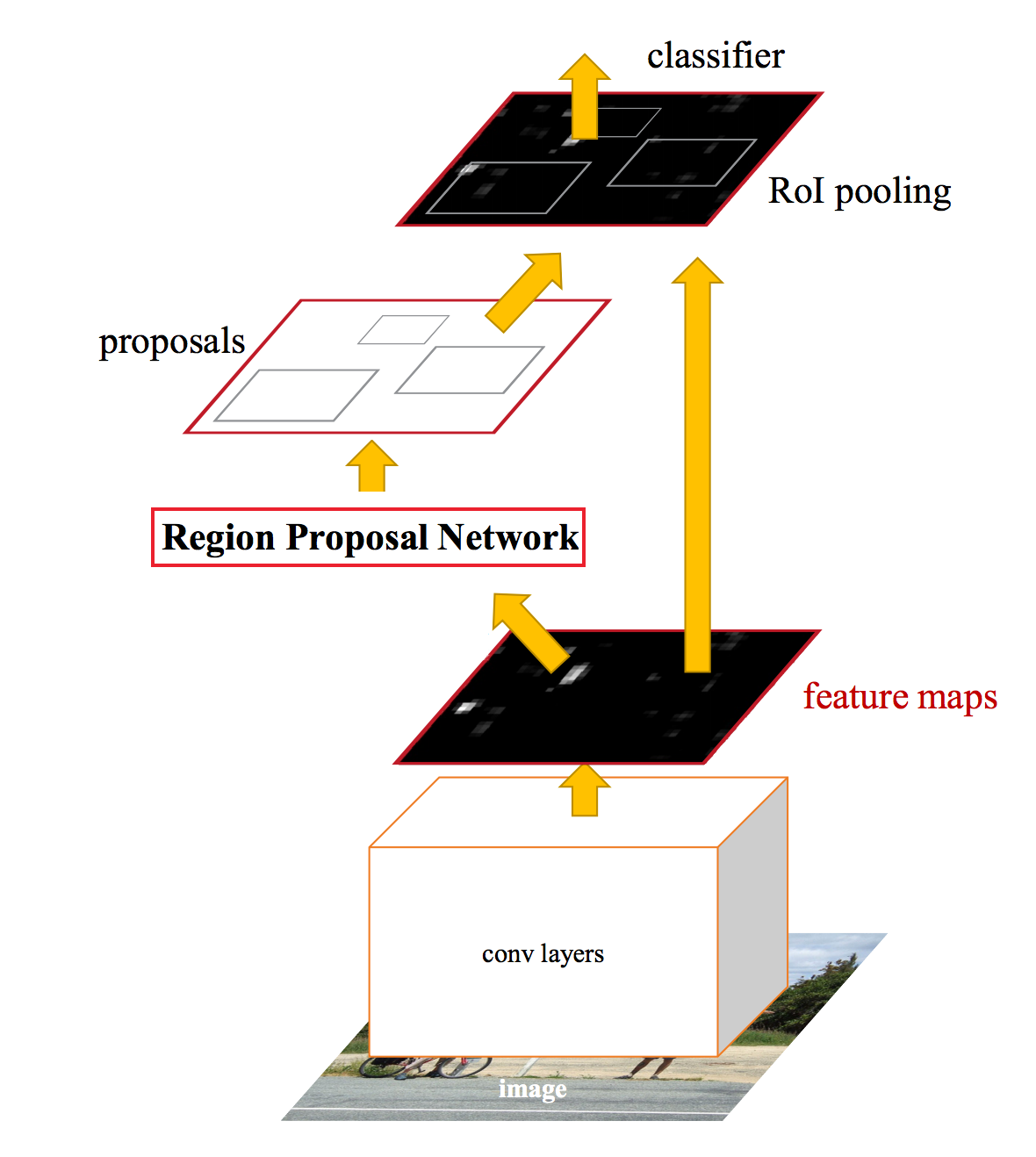
The difference between Fast R-CNN and Faster R-CNN is that we do not use a special region proposal method to create region proposals. Instead, we train a region proposal network that takes the feature maps as input and outputs region proposals. These proposals are then feed into the RoI pooling layer in the Fast R-CNN.
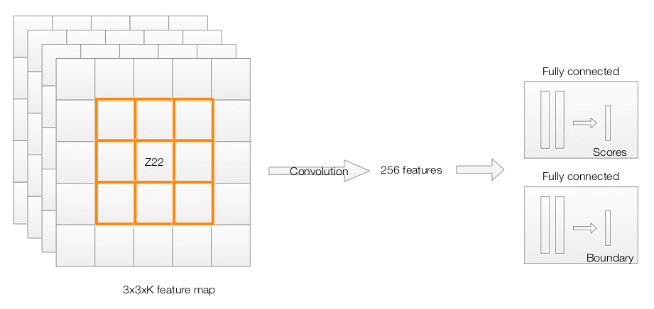
The region proposal network is a convolution network. The region proposal network uses the feature map of the “conv5” layer as input. It slides a 3x3 spatial windows over the features maps with depth K. For each sliding window, we output a vector with 256 features. Those features are feed into 2 fully-connected networks to compute:
- 2 scores representing how likely it is an object or non-object/background.
- A boundary box.
We then feed the region proposals to the RoI layer of the Fast R-CNN.
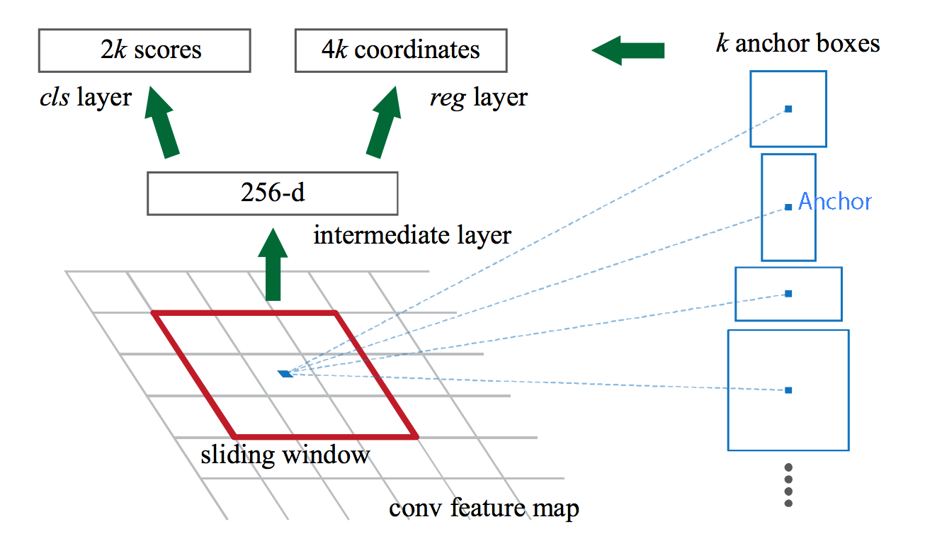
Multiple anchor boxes
In the example above, we generate 1 proposal per sliding window. The region proposal network can scale or change the aspect ratio of the window to generate more proposals. In Faster R-CNN, 9 anchor boxes (on the right) are generated per anchor.
Implementations
The implementations of Faster R-CNN can be found at: