“Memory network (MemNN) & End to end memory network (MemN2N), Dynamic memory network”
Memory network
Virtual assistances are pretty good at answering a one-line query but fail badly in carrying out a conversation. Here is a verbal exchange demonstrating the challenge ahead of us:
- Me: Can you find me some restaurants?
- Assistance: I find a few places within 0.25 mile. The first one is Caffé Opera on Lincoln Street. The second one is …
- Me: Can you make a reservation at the first restaurant?
- Assistance: Ok. Let’s make a reservation for the Sushi Tom restaurant on the First Street.
Why can’t the virtual assistance follow my instruction to book the Caffé Opera? It is because the virtual assistance does not remember our conversation and simply responses to our second query without the context of the previous conversation. Therefore, the best it can do is to find a restaurant that relates to the word “First”, and it finds a restaurant located on First Street. Memory networks address this issue by remembering information processed so far.
The description on the memory networks (MemNN) is based on Memory networks, Jason Weston etc.
Consider the follow sequence with a query “Where is the milk now?”:
- Joe went to the kitchen.
- Fred went to the kitchen.
- Joe picked up the milk.
- Joe traveled to the office.
- Joe left the milk.
- Joe went to the bathroom.
Storing information into the memory
First, we store all the sentences in the memory \(m\):
| Memory slot \(m_i\) | Sentence |
|---|---|
| 1 | Joe went to the kitchen. |
| 2 | Fred went to the kitchen. |
| 3 | Joe picked up the milk. |
| 4 | Joe traveled to the office. |
| 5 | Joe left the milk. |
| 6 | Joe went to the bathroom. |
Answering a query
To answer a query \(q\), we locate the sentence \(m_{o_1}\) that is most relevant to \(q\) computed by a score function \(s_o\). Then we combine this sentence \(m_{o_1}\) with \(q\) to form a new query \([q, m_{o_1}]\) and locate the next highest score sentence \(m_{o_2}\). At last, we form another query \([q, m_{o_1}, m_{o_2}]\). But we will not use it to query the next sentence. Instead, we query it with another score function \(s_r\) to locate a word \(w\). Let’s walk through this with our example above.
To answer the query \(q\) “where is the milk now?”, we compute our first inference based on:
\[o_1 = \underset{i=1, \dots, N}{\arg\max} s_0(q, m_{i})\]where \(s_{0}\) is a function that scores the match between an input \(x\) and \(m_{i}\), and \(o_1\) is the index to the memory \(m\) with the best match. Here, \(m_{o_1}\) is our best match in the first inference: “Joe left the milk.”
Then, we make a second inference based on \(\big[ q: \text{ "where is the milk now"} , m_{o_1}: \text{" Joe left the milk."} \big]\)
\[o_2 = \underset{i=1, \dots, N}{\arg\max} s_o(\big[ q, m_{o_{1}} \big], m_{i})\]where \(m_{o_2}\) will be “Joe traveled to the office.”.
We combine the query, and the inference results as \(o\):
\[o = \big[ q, m_{o_{1}} , m_{o_{2}} \big] = \big[ \text{ "where is the milk now"} , \text{" Joe left the milk."}, \text{" Joe travelled to the office."} \big]\]To generate a final response \(r\) from \(o\):
\[r = \underset{w \in W}{\arg\max} s_r(\big[ q, m_{o_{1}}, m_{o_{2}} \big], w)\]where \(W\) is all the words in the dictionary, and \(s_{r}\) is another function that scores the match between \(\big[ q, m_{o_{1}}, m_{o_{2}} \big]\) and a word \(w\). In our example, the final response \(r\) is the word “office”.
Encoding the input
We use bags of words to represent our input text. First, we start with a vocabulary of a size \(\left| W \right|\) .
To encode the query “where is the milk now” with bags of words:
| Vocabulary | … | is | Joe | left | milk | now | office | the | to | travelled | where | … |
|---|---|---|---|---|---|---|---|---|---|---|---|---|
| where is the milk now | … | 1 | 0 | 0 | 1 | 1 | 0 | 1 | 0 | 0 | 1 | … |
For better performance, we use 3 different set of bags to encode \(q\), \(m_{o_{1}}\) and \(m_{o_{2}}\) separately, i.e., we encode “Joe” in \(q\) as “Joe_1” and the same word in \(m_{o_{1}}\) as “Joe_2”:
\(q\): Where is the milk now?
\(m_{o_{1}}\): Joe left the milk.
\(m_{o_{2}}\): Joe travelled to the office.
To encode \(\big[ q, m_{o_{1}}, m_{o_{2}} \big]\) above, we use:
| … | Joe_1 | milk_1 | … | Joe_2 | milk_2 | … | Joe_3 | milk_3 | … | |
|---|---|---|---|---|---|---|---|---|---|---|
| 0 | 1 | 1 | 1 | 1 | 0 |
Hence, each sentence is converted to a bag of words of size \(3 \left| W \right|\) .
Compute the scoring function
We use word embeddings \(U\) to convert a sentence with a bag of words with size \(3 \left| W \right|\) into a dense word embedding with a size \(n\). We evaluate both score functions \(s_{o}\) and \(s_{r}\) with:
\[s_{o}(x, y) = Φ_{x}(x)^T{U_{o}}^TU_{o}Φ_{y}(y)\] \[s_{r}(x, y) = Φ_{x}(x)^T{U_{r}}^TU_{r}Φ_{y}(y)\]which embedding \(U_{o}\) and \(U_{r}\) are trained with a margin loss function, and \(Φ(m_i)\) converts the sentence \(m_i\) into a bag of words.
Margin loss function
We will train the parameters in \(U_{o}\) and \(U_{r}\) with the marginal loss function:
\[\sum_{\bar{f}\neq m_{o_{1}}} \max(0, γ - s_{o}(x, m_{o_{1}}) + s_{o}(x, \bar{f})) +\] \[\sum_{\bar{f}\neq m_{o_{2}}} \max(0, γ - s_{o}(\big[ x, m_{o_{1}} \big], m_{o_{2}} ) + s_{o}(\big[ x, m_{o_{1}} \big], \bar{f'})) +\] \[\sum_{\bar{r}\neq r} \max(0, γ - s_{r}(\big[ x, m_{o_{1}}, m_{o_{2}} \big], r ) + s_{r}(\big[ x, m_{o_{1}}, m_{o_{2}} \big], \bar{r} )\]where \(\bar{f}, \bar{f'}\) and \(\bar{r}\) are other possible predictions other than the true label. i.e. we add a margin loss if the score of the wrong answers are larger than the score of the ground truth minus \(γ\).
Huge memory networks
For a system with huge memory, computing every score for each memory entry is expensive. Alternatively, after computing the word embedding \(U_{0}\), we apply K-clustering to divide the word embedding space into K clusters. We map each input \(x\) into its corresponding cluster and perform inference within that cluster space only instead of the whole memory space.
End to end memory network (MemN2N)
The description, as well as the diagrams, on the end to end memory networks (MemN2N) are based on End-To-End Memory Networks, Sainbayar Sukhbaatar etc.
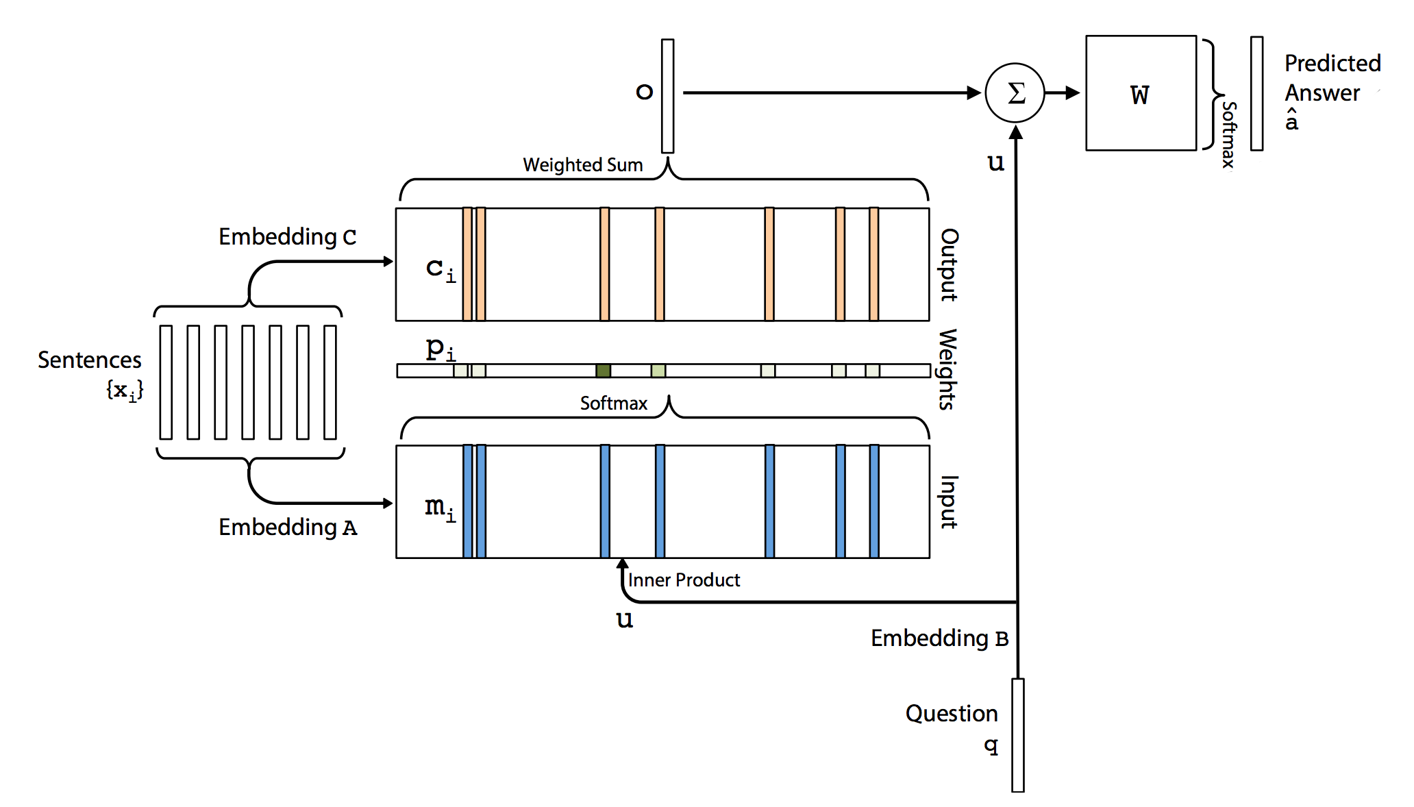
We start with a query “where is the milk now?”. It is encoded with bags of words using a vector of size \(V\). (which \(V\) is the size of the vocabulary.) In the simplest case, we use Embedding \(B\) (\(d \times V\)) to convert the vector to a word embedding of size d.
\[u = embedding_B(q)\]For each memory entry \(x_{i}\), we use another Embedding \(A\) (\(d \times V\)) to convert it to \(m_{i}\) of size d.
\[m_{i} = embedding_A(x_{i})\]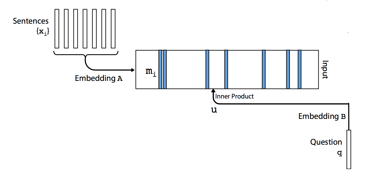
The match between \(u\) and each memory \(m_{i}\) is computed by taking the inner product followed by a softmax:
\[p_{i} = softmax(u^T m_{i}).\]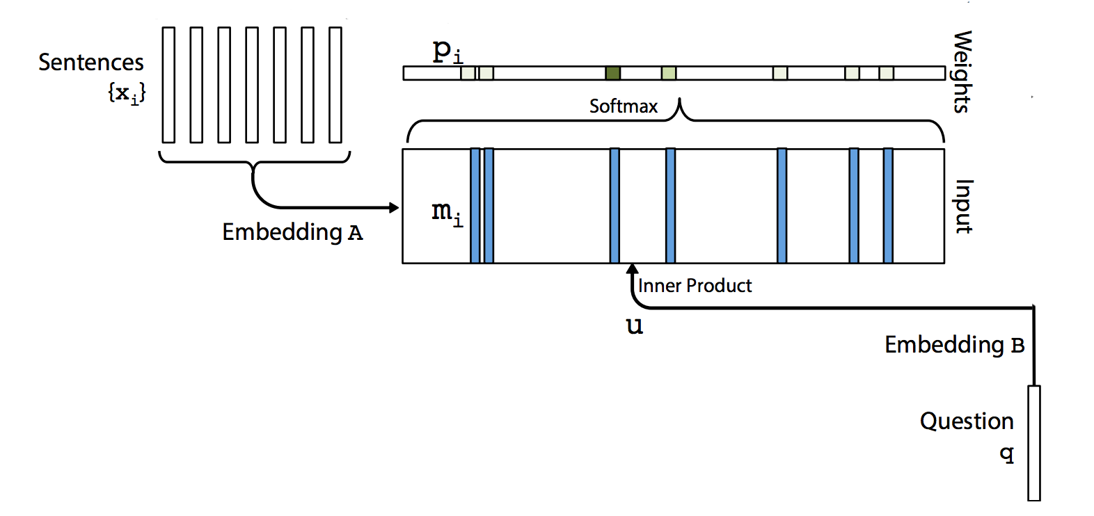
We use a third Embedding \(C\) to encode \(x_{i}\) as \(c_{i}\)
\[c_{i} = embedding_C(x_{i})\]The output is computed as:
\[o = \sum_{i} p_{i} c_{i} .\]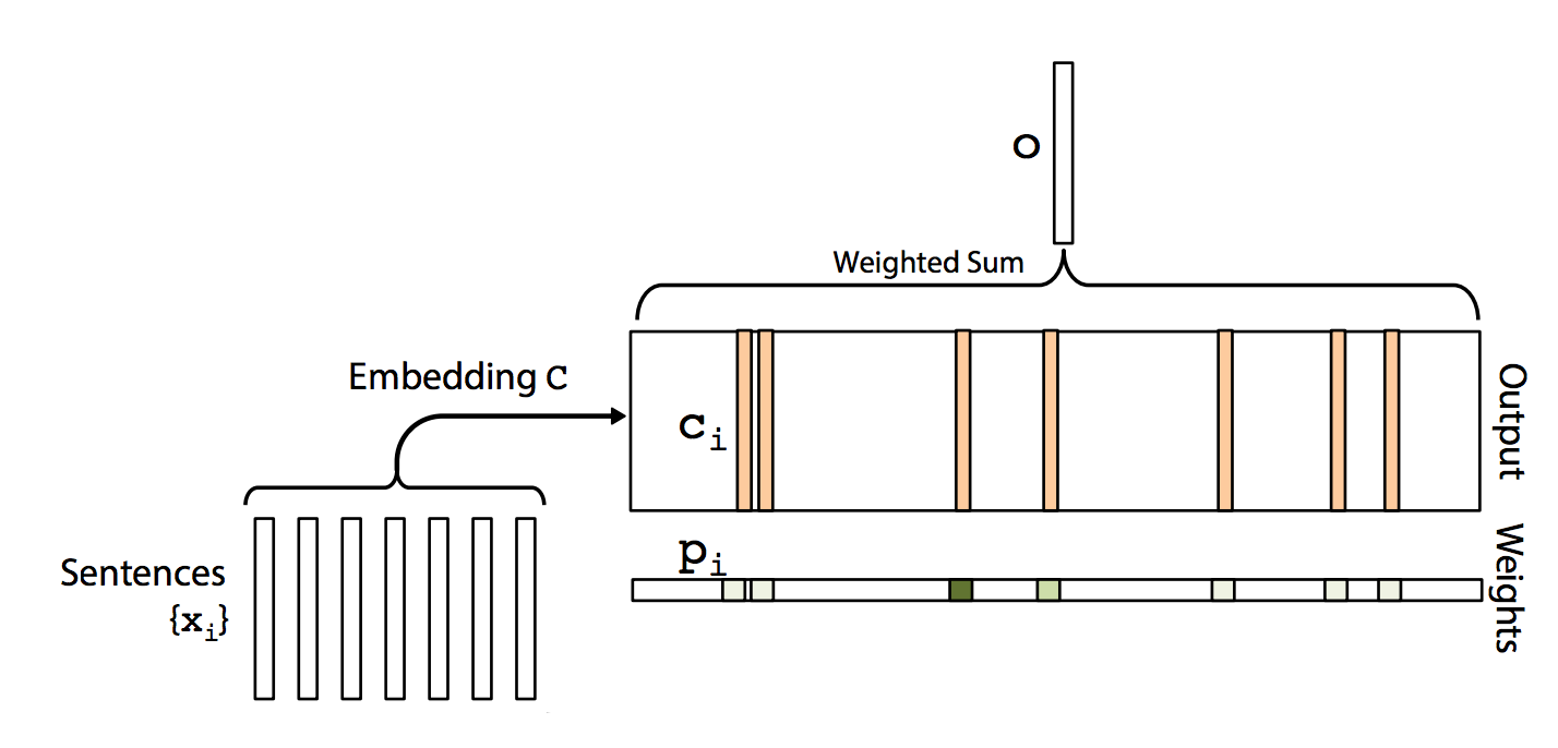
We multiply the sum of \(o\) and \(u\) with matrix W (\(V \times d\)). The result is passed to a softmax function to predict the final answer.
\[\hat{a} = softmax(W(o + u))\]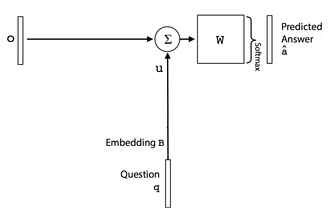
Here, we combine all the steps into one diagram:
Multiple layer
Similar to RNN, we can stack multiple layers to form a complex network. At each layer \(i\), it has its own embedding \(A_{i}\) and embedding \(C_{i}\). The input at layer \(k+1\) is computed by:
\[u^{k+1} = u^k + o^k.\]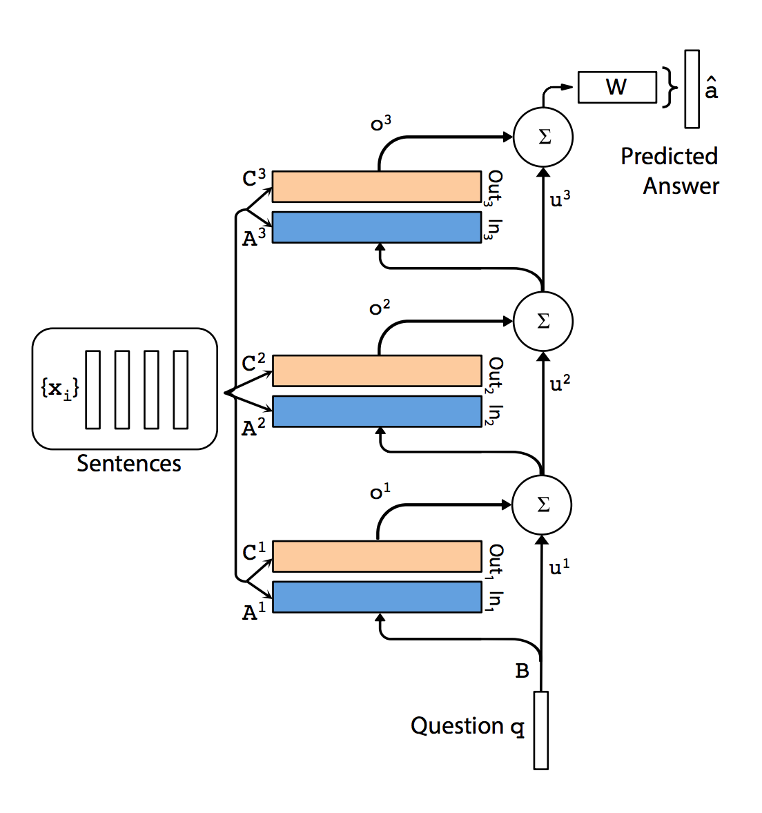
Language model
We can use MemN2N as a language model. For example, we parse the document “Declaration of Independence”: “We hold these truths to be self-evident, that all men are created equal, that they are endowed by their Creator with certain unalienable Rights, that among these are Life, Liberty and the pursuit of Happiness.” Instead of 1 sentence per memory entry, we store only one word per entry as follows:
| Memory slot \(m_i\) | Word |
|---|---|
| 1 | We |
| 2 | hold |
| 3 | these |
| 4 | truths |
| 5 | to |
| 6 | be |
| 7 | … |
The purpose of the language model is to predict say the word 7 “self-evident” above.
Changes are made according to sections described in the MemN2N paper.
- There are no query. We try to find the next word. Not a response to a query. Hence, we do not need embedding B and we just fill \(u\) with a constant say 0.1.
- We use multiple layers but we use the same embedding \(A\) for all layers. We use a separate embedding \(B\) for all layer.
- We add a temporal term into our embedding to record the ordering of the words in the memory. (Section 4.1)
- We multiple \(u\) with a linear vector before adding to o. (Section 2)
- To aid training, we apply ReLU operations to half of the units in each layer. (Section 5)
Here is the code of building the embedding \(A, C\), \(m_i\), \(c_i\), \(p\), \(o\) and \(\hat{a}\).
def build_memory(self):
    self.A = tf.Variable(tf.random_normal([self.nwords, self.edim], stddev=self.init_std)) # Embedding A for sentences
    self.C = tf.Variable(tf.random_normal([self.nwords, self.edim], stddev=self.init_std)) # Embedding C for sentences
    self.H = tf.Variable(tf.random_normal([self.edim, self.edim], stddev=self.init_std))   # Multiple it with u before adding to o

    # Sec 4.1: Temporal Encoding to capture the time order of the sentences.
    self.T_A = tf.Variable(tf.random_normal([self.mem_size, self.edim], stddev=self.init_std))
    self.T_C = tf.Variable(tf.random_normal([self.mem_size, self.edim], stddev=self.init_std))

    # Sec 2: We are using layer-wise (RNN-like) which the embeddings for each layers are sharing the parameters.
    # (N, 100, 150) m_i = sum A_ij * x_ij + T_A_i
    m_a = tf.nn.embedding_lookup(self.A, self.sentences)
    m_t = tf.nn.embedding_lookup(self.T_A, self.T)
    m = tf.add(m_a, m_t)

    # (N, 100, 150) c_i = sum C_ij * x_ij + T_C_i
    c_a = tf.nn.embedding_lookup(self.C, self.sentences)
    c_t = tf.nn.embedding_lookup(self.T_C, self.T)
    c = tf.add(c_a, c_t)

	# For each layer
    for h in range(self.nhop):
        u = tf.reshape(self.u_s[-1], [-1, 1, self.edim])
        scores = tf.matmul(u, m, adjoint_b=True)
        scores = tf.reshape(scores, [-1, self.mem_size])

        P = tf.nn.softmax(scores)     # (N, 100)
        P = tf.reshape(P, [-1, 1, self.mem_size])

        o = tf.matmul(P, c)
        o = tf.reshape(o, [-1, self.edim])

        # Section 2: We are using layer-wise (RNN-like), so we multiple u with H.
        uh = tf.matmul(self.u_s[-1], self.H)
        next_u = tf.add(uh, o)

        # Section 5:  To aid training, we apply ReLU operations to half of the units in each layer.
        F = tf.slice(next_u, [0, 0], [self.batch_size, self.lindim])
	    G = tf.slice(next_u, [0, self.lindim], [self.batch_size, self.edim-self.lindim])
        K = tf.nn.relu(G)
        self.u_s.append(tf.concat(axis=1, values=[F, K]))

    self.W = tf.Variable(tf.random_normal([self.edim, self.nwords], stddev=self.init_std))
    z = tf.matmul(self.u_s[-1], self.W)
Compute the cost and building the optimizer with gradient clipping
self.loss = tf.nn.softmax_cross_entropy_with_logits(logits=z, labels=self.target)

self.lr = tf.Variable(self.current_lr)
self.opt = tf.train.GradientDescentOptimizer(self.lr)

params = [self.A, self.C, self.H, self.T_A, self.T_C, self.W]
grads_and_vars = self.opt.compute_gradients(self.loss, params)
clipped_grads_and_vars = [(tf.clip_by_norm(gv[0], self.max_grad_norm), gv[1]) \
                                   for gv in grads_and_vars]

inc = self.global_step.assign_add(1)
with tf.control_dependencies([inc]):
      self.optim = self.opt.apply_gradients(clipped_grads_and_vars)
Training
def train(self, data):
    n_batch = int(math.ceil(len(data) / self.batch_size))
    cost = 0

    u = np.ndarray([self.batch_size, self.edim], dtype=np.float32)      # (N, 150) Will fill with 0.1
    T = np.ndarray([self.batch_size, self.mem_size], dtype=np.int32)    # (N, 100) Will fill with 0..99
    target = np.zeros([self.batch_size, self.nwords])                   # one-hot-encoded
    sentences = np.ndarray([self.batch_size, self.mem_size])

    u.fill(self.init_u)   # (N, 150) Fill with 0.1 since we do not need query in the language model.
    for t in range(self.mem_size):   # (N, 100) 100 memory cell with 0 to 99 time sequence.
       T[:,t].fill(t)

    for idx in range(n_batch):
        target.fill(0)      # (128, 10,000)
        for b in range(self.batch_size):
            # We random pick a word in our data and use that as the word we need to predict using the language model.
            m = random.randrange(self.mem_size, len(data))
            target[b][data[m]] = 1                       # Set the one hot vector for the target word to 1

            # (N, 100). Say we pick word 1000, we then fill the memory using words 1000-150 ... 999
            # We fill Xi (sentence) with 1 single word according to the word order in data.
           sentences[b] = data[m - self.mem_size:m]

            _, loss, self.step = self.sess.run([self.optim,
                                                self.loss,
                                                self.global_step],
                                                feed_dict={
                                                    self.u: u,
                                                    self.T: T,
                                                    self.target: target,
                                                    self.sentences: sentences})
            cost += np.sum(loss)

    return cost/n_batch/self.batch_size
The initialization code and creating placeholder:
class MemN2N(object):
    def __init__(self, config, sess):
        self.nwords = config.nwords         # 10,000
        self.init_u = config.init_u         # 0.1 (We don't need a query in language model. So set u to be 0.1
        self.init_std = config.init_std     # 0.05
        self.batch_size = config.batch_size # 128
        self.nepoch = config.nepoch         # 100
        self.nhop = config.nhop             # 6
        self.edim = config.edim             # 150
        self.mem_size = config.mem_size     # 100
        self.lindim = config.lindim         # 75
        self.max_grad_norm = config.max_grad_norm   # 50

        self.show = config.show
        self.is_test = config.is_test
        self.checkpoint_dir = config.checkpoint_dir

        if not os.path.isdir(self.checkpoint_dir):
            raise Exception(" [!] Directory %s not found" % self.checkpoint_dir)

        # (?, 150) Unlike Q&A, the language model do not need a query (or care what is its value).
        # So we bypass q and fill u directly with 0.1 later.
        self.u = tf.placeholder(tf.float32, [None, self.edim], name="u")

        # (?, 100) Sec. 4.1, we add temporal encoding to capture the time sequence of the memory Xi.
        self.T = tf.placeholder(tf.int32, [None, self.mem_size], name="T")

        # (N, 10000) The answer word we want. (Next word for the language model)
        self.target = tf.placeholder(tf.float32, [self.batch_size, self.nwords], name="target")

        # (N, 100) The memory Xi. For each sentence here, it contains 1 single word only.
        self.sentences = tf.placeholder(tf.int32, [self.batch_size, self.mem_size], name="sentences")

        # Store the value of u at each layer
        self.u_s = []
        self.u_s.append(self.u)
The full source code is in github with original code based on https://github.com/carpedm20/MemN2N-tensorflow.
Dynamic memory network
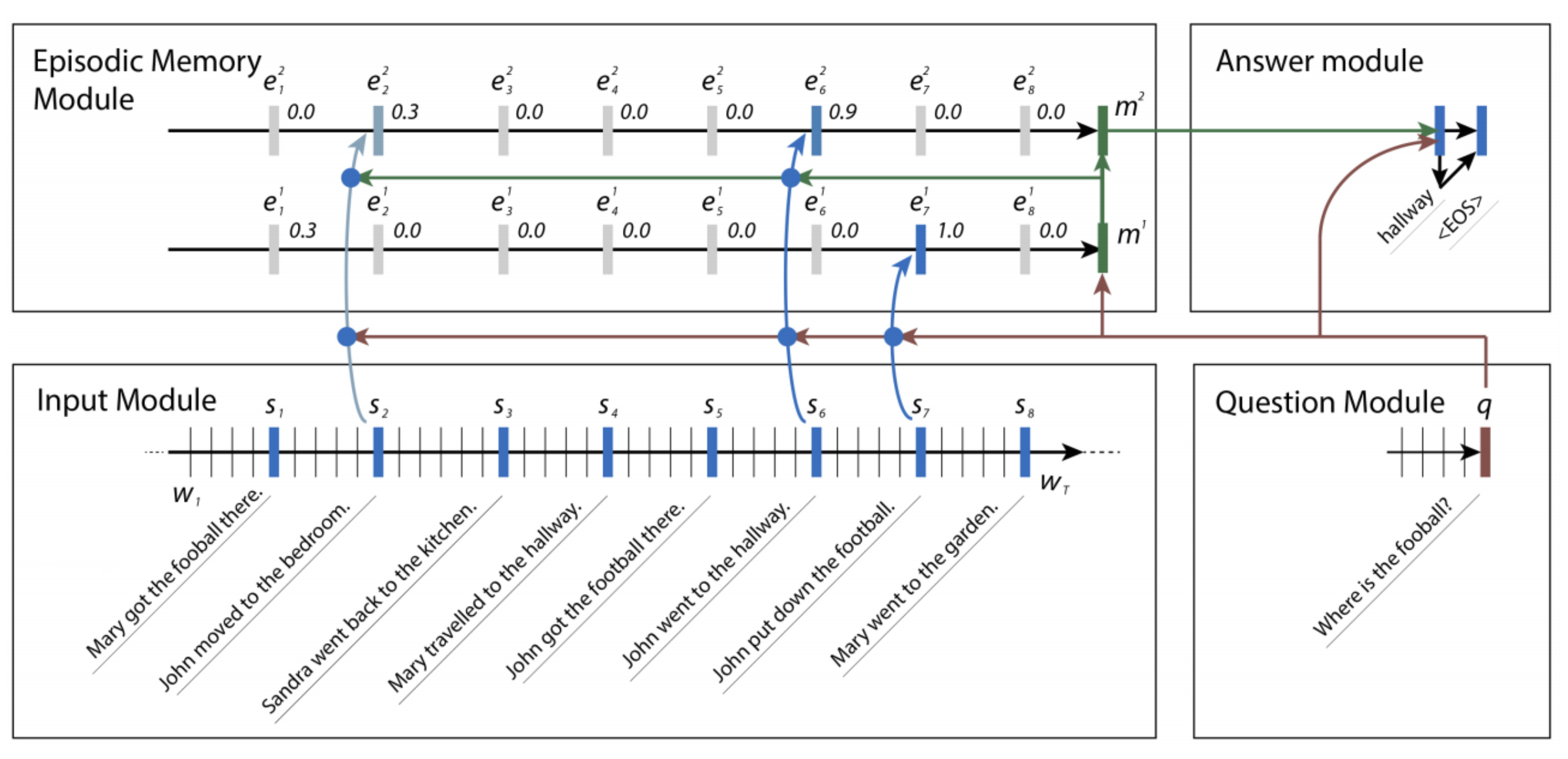
Sentence
Sentence is processed by a GRU which the last hidden state is used for the memory module.
Question module
\[\begin{split} q_t & = GRU(v_t, q_{t-1})\\ \end{split}\]Episodic memory module
\[\begin{split} h^t_i & = g^t_i GRU(s_i, h^t_{i-1}) + (1-g^t_i) h^t_{i-1} \\ \end{split}\]which \(s_i\) is the sentence \(i\). \(h^t_i\) is the hidden state at time step t after after processing sentence \(i\). The last hidden state of \(h^t_i\) is \(m^{'}\).
Gate
\(g^t_i\) is the gate control on what new information is added to \(h^t\). It is open if it is relevant to the question or memory \(m^{'}\). We first form a new feature set by concatenating:
\[\begin{split} z^t_i &=[s_i \circ q, s_i \circ m^{t-1}, \vert s_i - q \vert, \vert s_i - m^{t-1}\vert ] \\ \end{split}\]The gate is computed as:
\[\begin{split} Z ^t_i &= W^2 \tanh (W^1 z^t_i + b^1) + b^2 \\ g^t_i &= \frac{exp(Z^t_i)}{\sum_k exp(Z^t_k)} \\ \end{split}\]Answer module
After \(m^{'}\) is computed, the relevant facts are summarized in another GRU. If the summary is not sufficient to answer the question, we move to \(t+1\) in the memory module.
\[\begin{split} a_t &= GRU([y_{t-1}], a_{t-1}) \\ y_t &= softmax(W^a a_t) \\ \end{split}\]