“RNN, LSTM and GRU tutorial”
Recurrent Neural Network (RNN)
If convolution networks are deep networks for images, recurrent networks are networks for speech and language. For example, both LSTM and GRU networks based on the recurrent network are popular for the natural language processing (NLP). Recurrent networks are heavily applied in Google home and Amazon Alexa. To illustrate the core ideas, we look into the Recurrent neural network (RNN) before explaining LSTM & GRU.
In deep learning, we model h in a fully connected network as:
\[h = f(X_i)\]where \(X_i\) is the input.
For time sequence data, we also maintain a hidden state representing the features in the previous time sequence. Hence, to make a word prediction at time step t in speech recognition, we take both input \(X_t\) and the hidden state from the previous time step \(h_{t-1}\) to compute \(h_t\):
\[h_t = f(x_t, h_{t-1})\]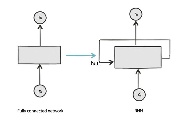
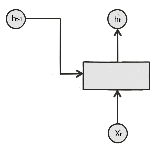
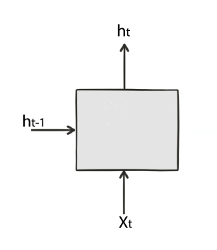
We can unroll the time step \(t\) which takes the hidden state \(h_{t-1}\) and input \(X_t\) to compute \(h_t\).
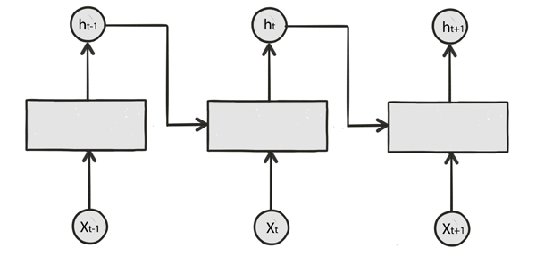
To give another perspective, we unroll a RNN from time step \(t-1\) to \(t+1\):
In RNN, \(h\) servers 2 purposes: the hidden state for the previous sequence data as well as making a prediction. In the following example, we multiply \(h_t\) with a matrix \(W\) to make a prediction for \(Y\). Through the multiplication with a matrix, \(h_t\) make a prediction for the word that a user is pronouncing.
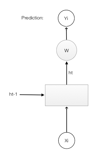
RNN makes prediction based on the hidden state in the previous timestep and current input. \(h_t = f(x_t, h_{t-1})\)
Create image caption using RNN
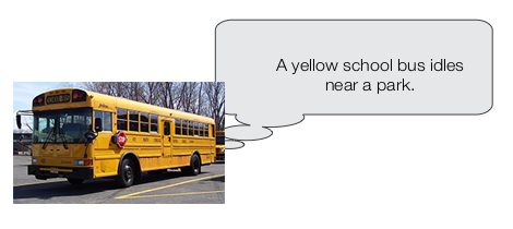
Let’s study a real example to study RNN in details. We want our system to automatically provide captions by simply reading an image. For example, we input a school bus image into a RNN and the RNN produces a caption like “A yellow school bus idles near a park.”
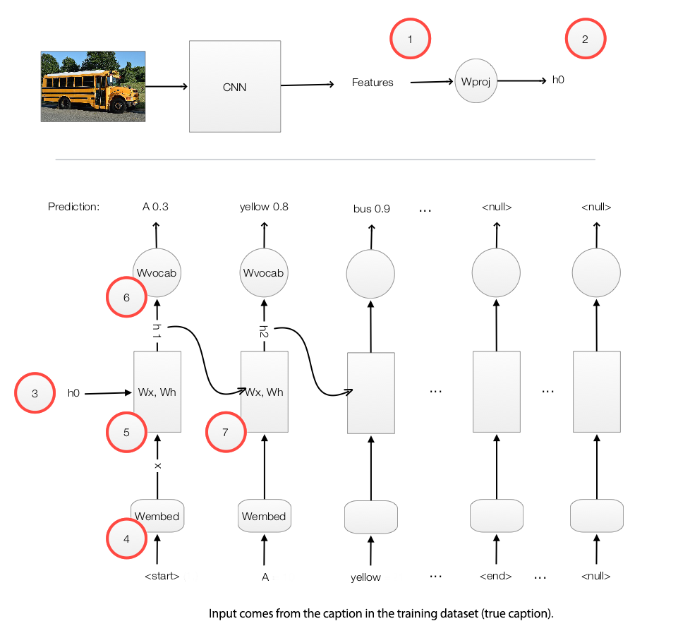
During the RNN training, we
- Use a CNN network to capture features of an image.
- Multiple the features with a trainable matrix to generate \(h_0\).
- Feed \(h_0\) to the RNN.
- Use a word embedding lookup table to convert a word to a word vector \(X_1\). (a.k.a word2vec)
- Feed the word vector and \(h_0\) to the RNN. \(h_1 = f(X_1, h_0)\)
- Use a trainable matrix to map \(h\) to scores which predict the next word in our caption.
- Move to the next time step with \(h_1\) and the word “A” as input.
Capture image features
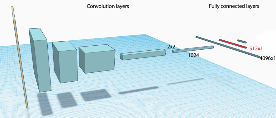
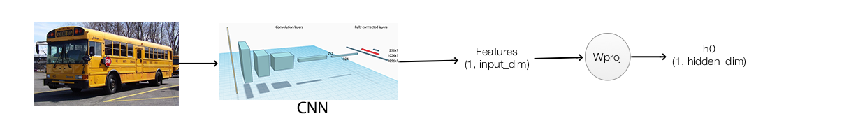
We pass the image into a CNN and use one of the activation layer in the fully connected (FC) network to initialize the RNN. For example, in the picture below, we pick the input of the second FC layer to compute the initial state of the RNN \(h_0\).
We multiply the CNN image features with a trainable matrix to compute \(h_0\) for the first time step 1.
With \(h_0\), we compute \(h_1 = f(h_0, X_1)\) for time step 1.
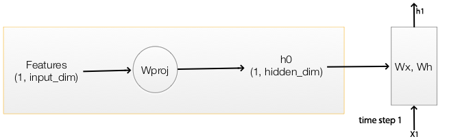
We use a CNN to extract image features. Multiple it with a trainable matrix for the initial hidden state \(h_0\).
Code in computing h0
Define the shape of CNN image features (N, 512) and h (N, 512):
input_dim   = 512   # CNN features dimension: 512
hidden_dim  = 512   # Hidden state dimension: 512
Define a matrix to project the CNN image features to \(h_0\).
# W_proj: (input_dim, hidden_dim)
W_proj  = np.random.randn(input_dim, hidden_dim)
W_proj /= np.sqrt(input_dim)
b_proj  = np.zeros(hidden_dim)
Compute \(h_0\) by multiply the image features with \(W_{proj}\).
# Initialize CNN -> hidden state projection parameters
# h0: (N, hidden_dim)
h0 = features.dot(W_proj) + b_proj
We initialize \(h_0 = W_{proj} \cdot x_{cnn}+ b\) .
Map words to RNN
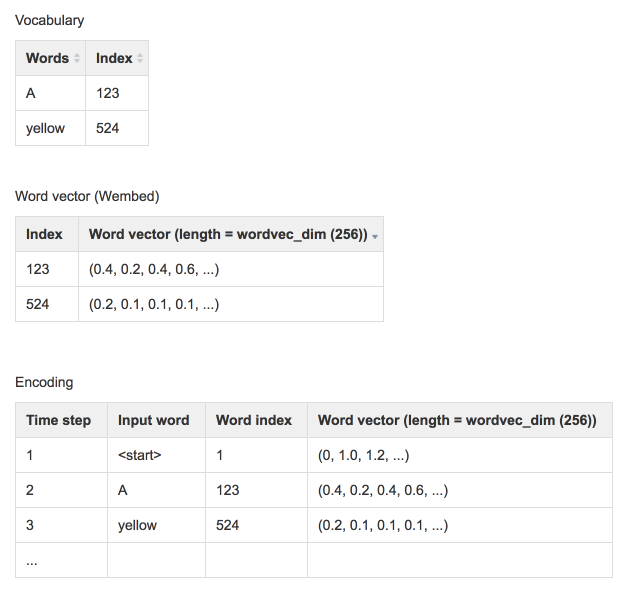
Our training data contains both the images and captions (the true labels). It also has a dictionary which maps a vocabulary word to an integer index. Caption words in the dataset are stored as word indexes using the dictionary. For example, the caption “A yellow school bus idles near a park.” can be represented as “1 5 3401 3461 78 5634 87 5 111 2” which 1 represents the “start” of a caption, 5 represents ‘a’, 3401 represents ‘yellow’, … and 2 represents the “end” of a caption.
The RNN does not use the word index. The word index does not contain information about the semantic relationship between words. We map a word to a higher dimensional space such that we can encode semantic relationship between words. For example, if we encode the word “father” as (0.2, 0.3, 0.1, …) we should expect the word “mother” to be close by say (0.3, 0.3, 0.1, …). The vector distance between the word “Paris” and “France” should be similar to the one between “Seoul” and “Korea”. The encoding method word2vec provides a mechanism to convert a word to a higher dimensional space. We use a word embedding lookup table \(W_{embed}\) to convert a word index to a vector of length wordvec_dim. This embedding table is trained together with the caption creating network instead of training them independently (end-to-end training).
We train the word embedding table together with the caption creation network.
The RNN will take this vector \(X_t\) and \(h_{t-1}\) to compute \(h_t\)
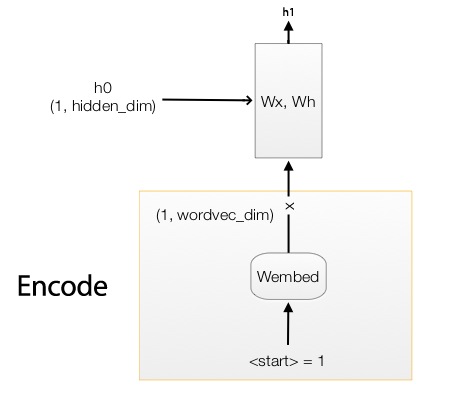
word2vec encodes words to higher dimensional space that provides semantic relationships that we can manipulate as vectors.
When we create the training data, we encodes words to the corresponding word index using a vocabulary dictionary. The encoded data will then be saved. During training, we read the saved dataset and use word2vec to convert the word index to a word vector.
Here is the code to convert an input caption word to the word vector x.
wordvec_dim = 256 # Convert a work index to a vector of 256 numbers.
Randomly initialize W which we will train it with the RNN together.
W_embed  = np.random.randn(vocab_size, wordvec_dim)
W_embed /= 100
Look up the word vector from a word index using the lookup table (W)
# T = 16: Number of unroll time step.
# captions:    (N, T+1) The caption represent "<start> A yellow school bus idles near a park <end> <null> ... <null>" represent in word index.
# captions_in  (N, T) The caption feed into the RNN (X) = captions without the last word.
# captions_out (N, T) The true caption output: the caption without "<start>"

# W_embed (vocab_size, wordvec_dim)
# captions_in: (N, T) each captions_in contain at most 16 words.
# x: (N, T, wordvec_dim)
x, cache_embed = word_embedding_forward(captions_in, W_embed)
def word_embedding_forward(x, W):
  out, cache = None, None
  N, T = x.shape
  V, D = W.shape
  out = W[x]
  cache = (V, x)
  return out, cache
Use \(W_{embed}\) to convert a word to a word vector.
RNN
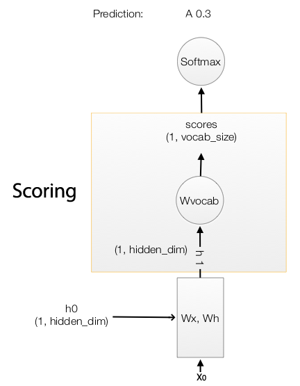
We pass the word vector \(X_0\) into the RNN cell to compute the next hidden state \(h_{t}\):
\[\begin{align} state & = W_x x_t + W_h h_{t-1} + b \\ h_{t} &= \tanh(state) \\ \end{align}\]The output of the RNN \(h_1\) is then multiply with \(W_{vocab}\) to generate scores for each word in the vocabulary. For example, if we have 10004 words in the vocabulary, it generates 10004 scores predicting the likeliness of each word to be the next word in the caption. With the true caption in the training dataset and the scores computed, we calculate the softmax loss of the RNN. We apply gradient descent to optimize the trainable parameters.
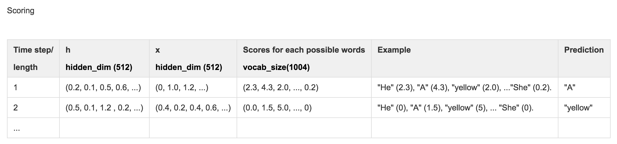
We compute \(h_t\) by feeding the RNN cell with \(X_t\) and \(h_{t-1}\). We then map \(h_t\) to scores which are used to compute the softmax cost.
# h: (N, 16, hidden_dim)
# Wx: (wordvec_dim, hidden_dim)
# Wh: (hidden_dim, hidden_dim)
h, cache_rnn = rnn_forward(x, h0, Wx, Wh, b)

# W_vocal: (hidden_dim, vocab_size 1004)
# scores: (N, 16, vocab_size 1004)
scores, cache_scores = temporal_affine_forward(h, W_vocab, b_vocab)
loss, dscores = temporal_softmax_loss(scores, captions_out, mask)
rnn_forward
“rnn forward” is the RNN layer that compute \(h_1, h_2, \cdots, h_t\)
h, cache_rnn = rnn_forward(x, h0, Wx, Wh, b)
rnn_forward unroll the RNN by T time steps and compute \(h_t\) by calling the RNN cell “rnn_step_forward”. At each step, it takes \(h_{t-1}\) from the previous step and use the true captions provided by the training set to lookup \(X_t\). Note, we use the true label instead of the highest score word from previous time step as input.
def rnn_forward(x, h0, Wx, Wh, b):
  """
    x: the true caption
  """
  h, cache = None, None
  N, T, D = x.shape

  # H is the dimension of the hidden state
  H = h0.shape[1]

  # h hold all the hidden states in all T steps
  h = np.zeros((N, T, H))

  state = {}
  state[-1] = h0

  cache_step = [None] * T

  # Unroll T steps
  for t in range(T):
    # Get the true label at t
    xt = x[:, t, :]
    # Compute one RNN step
    state[t], cache_step[t] = rnn_step_forward(xt, state[t-1], Wx, Wh, b)
    # Store the hidden state for time step t
    h[:, t, :] = state[t]

  cache = (cache_step, D)
  return h, cache
In each RNN time step, we compute:
\[\begin{align} state & = W_x x_t + W_h h_{t-1} + b \\ h_{t} &= \tanh(state) \\ \end{align}\]def rnn_step_forward(x, prev_h, Wx, Wh, b):
next_h, cache = None, None
state = np.dot(x, Wx) + np.dot(prev_h, Wh) + b
next_h = np.tanh(state)
cache = x, prev_h, Wx, Wh, state
return next_h, cache
We unroll RNN for T steps, each computing \(\tanh(Wx + b)\).
Scores
After finding \(h_t\), we compute the scores by:
\[score = W_{vocab} * h_t\] def temporal_affine_forward(x, w, b):
N, T, D = x.shape
M = b.shape[0]
out = x.reshape(N * T, D).dot(w).reshape(N, T, M) + b
cache = x, w, b, out
return out, cache
We compute score to locate the next most likely caption word.
Softmax cost
For each word in the vocabulary (1004 words), we predict their probabilities of being the next caption word using softmax. Without changing the result, we subtract it with the maximum score for better numeric stability.
\[softmax(z) = \frac{e^{z_i}}{\sum e^{z_c}} = \frac{e^{z_i - m}}{\sum e^{z_c - m}}\]We then compute the softmax loss (negative log likelihood) and the gradient.
\[\begin{align} J(w) &= - \sum_{i=1}^{N} \log p(\hat{y}^i = y^i \vert x^i, w ) \\ \nabla_{z_i} J &= \begin{cases} p - 1 \quad & \hat{y} = y \\ p & \text{otherwise} \end{cases} \end{align}\]def temporal_softmax_loss(x, y, mask):
N, T, V = x.shape
x_flat = x.reshape(N * T, V)
y_flat = y.reshape(N * T)
mask_flat = mask.reshape(N * T)
# We compute the softmax. We minus the score with a max for better numerical stability.
probs = np.exp(x_flat - np.max(x_flat, axis=1, keepdims=True))
probs /= np.sum(probs, axis=1, keepdims=True)
# Compute the softmax loss: negative log likelihood aka cross entropy loss
loss = -np.sum(mask_flat * np.log(probs[np.arange(N * T), y_flat])) / N
# Compute the gradient
dx_flat = probs.copy()
dx_flat[np.arange(N * T), y_flat] -= 1
dx_flat /= N
dx_flat *= mask_flat[:, None]
dx = dx_flat.reshape(N, T, V)
return loss, dx
Time step 0
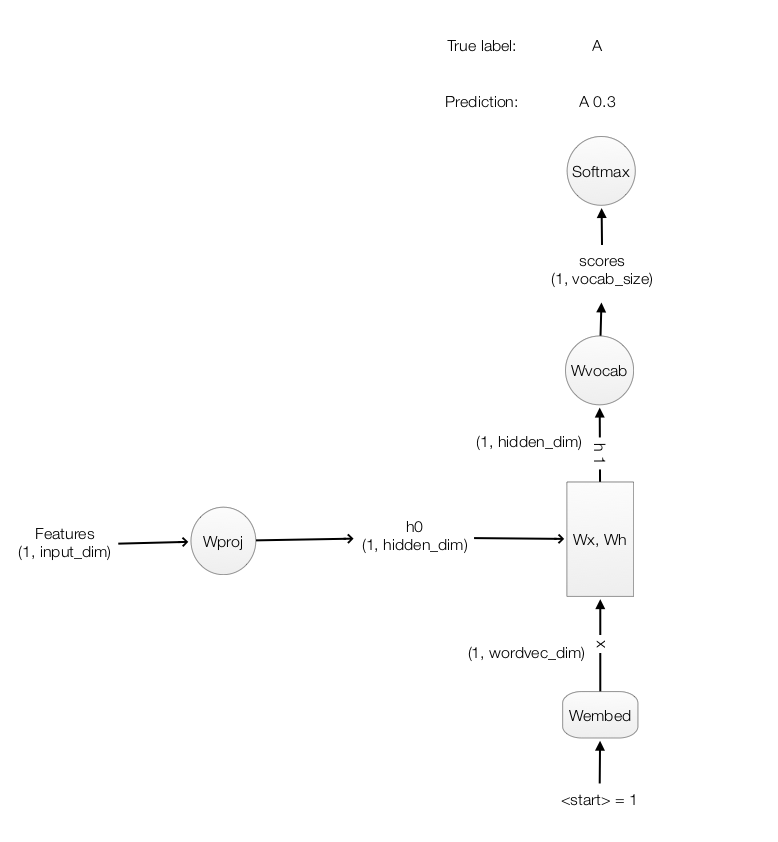
Here, we recap how we calculate \(h_0\) from the image features and use the true caption “start” to make a prediction \(h_1\) from the RNN. Then we compute the scores and the softmax loss.
Code listing for the forward feed, backpropagation and the loss.
  def loss(self, features, captions):
    # For training, say the caption is "<start> A yellow bus idles near a park"
    # captions_in is the Xt input: "<start> A yellow bus idles near a"
    # captions_out is the true label: "A yellow bus idles near a park"
    captions_in = captions[:, :-1]
    captions_out = captions[:, 1:]

    mask = (captions_out != self._null)

    # Retrieve the trainable parameters
    W_proj, b_proj = self.params['W_proj'], self.params['b_proj']
    W_embed = self.params['W_embed']
    Wx, Wh, b = self.params['Wx'], self.params['Wh'], self.params['b']
    W_vocab, b_vocab = self.params['W_vocab'], self.params['b_vocab']

    loss, grads = 0.0, {}
    # vocab_size = 1004
    # T          = 16
    #
    # features    : (N, input_dim)
    # W_proj      : (input_dim, hidden_dim)
    # h0          : (N, hidden_dim)
    #
    # x           : (N, T, wordvec_dim)
    # captions_in : (N, T) of word index
    # W-embed     : (vacab_size, wordvec_dim)
    #
    # h           : (N, 16, hidden_dim)
    # Wx          : (wordvec_dim, hidden_dim)
    # Wh          : (hidden_dim, hidden_dim)
    #
    # scores      : (N, 16, vocab_size)
    # W_vocab     : (hidden_dim, vocab_size)

    # Compute h0 from the image features.
    h0 = features.dot(W_proj) + b_proj

    # Find the word vector of the input caption word.
    x, cache_embed = word_embedding_forward(captions_in, W_embed)

    # Forward feed for the RNN
    h, cache_rnn = rnn_forward(x, h0, Wx, Wh, b)

    # Compute the scores for each words in the vocabulary
    scores, cache_scores = temporal_affine_forward(h, W_vocab, b_vocab)

    # Compute the softmax loss
    loss, dscores = temporal_softmax_loss(scores, captions_out, mask)

    # Perform the backpropagation
    dh, grads['W_vocab'], grads['b_vocab'] = temporal_affine_backward(dscores, cache_scores)
    dx, dh0, grads['Wx'], grads['Wh'], grads['b'] = rnn_backward(dh, cache_rnn)
    grads['W_embed'] = word_embedding_backward(dx, cache_embed)
    grads['b_proj'] = np.sum(dh0, axis=0)
    grads['W_proj'] = features.T.dot(dh0)

    return loss, grads
Use softmax cost to train the network.
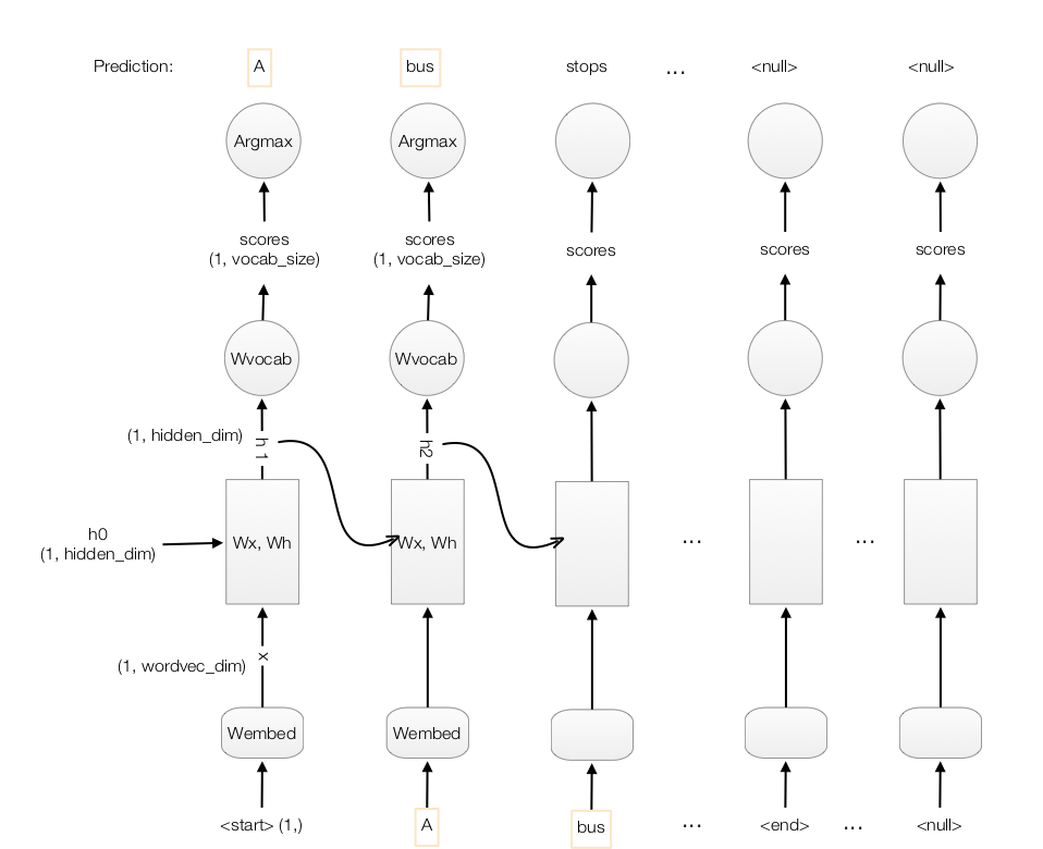
Making prediction
To generate captions automatically, we will use the CNN to generate image features and map it to \(h_0\) with \(W_{proj}\).

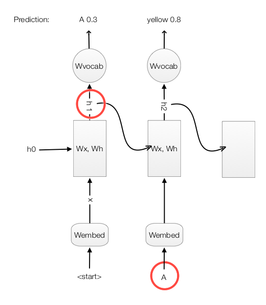
At time step 1, we feed the RNN with the input “start” to get the word vector \(X_1\). The RNN computes the value \(h_1\) which later multiplies with \(W_{vocab}\) to generate scores for each word in the vocabulary. We select the word with the highest score for the first word in the caption (say, “A”). Unlikely training, we use this word as the next time step input. With \(h_1\) and the highest score word “A” in time step 1, we go through the RNN step again and made the second prediction “bus” at time step 2.
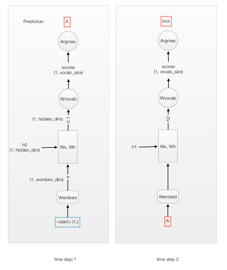
We compute the score and set the input for the next time step to be the word with the highest score.
scores, _ = affine_forward(next_h, W_vocab, b_vocab)
captions[:, t] = scores.argmax(axis=1)
prev_word = captions[:, t].reshape(N, 1)
Here is the full code making the prediction with comments:
def sample(self, features, max_length=30):
    N = features.shape[0]
    captions = self._null * np.ones((N, max_length), dtype=np.int32)

    # Retrive all trainable parameters
    W_proj, b_proj = self.params['W_proj'], self.params['b_proj']
    W_embed = self.params['W_embed']
    Wx, Wh, b = self.params['Wx'], self.params['Wh'], self.params['b']
    W_vocab, b_vocab = self.params['W_vocab'], self.params['b_vocab']

    # N is the size of the data to test
    # prev_word : (N, 1)
    #
    # next_h    : (N, hidden_dim)
    # features  : (N, input_dim)
    # W_proj    : (input_dim, hidden_dim)
    #
    # embed     : (N, 1, wordvec_dim)
    # W-embed   : (vacab_size, wordvec_dim)
    #
    # next_c    : (N, hidden_dim*4) for LSTM
    #
    # scores    : (N, vocab_size)
    # W_vocab     : (hidden_dim, vocab_size)
    #
    # captions  : (N, max_length)

    # Set the first word as "<start>"
    prev_word = self._start * np.ones((N, 1), dtype=np.int32)

    # Compute h0
    next_h, affine_cache = affine_forward(features, W_proj, b_proj)

    H, _ = Wh.shape
    # for each time step
    for t in range(max_length):
      # Compute the word vector.
      embed, embed_cache = word_embedding_forward(prev_word, W_embed)
      # Compute h from the RNN
      next_h, cache = rnn_step_forward(np.squeeze(embed), next_h, Wx, Wh, b)
      # Map h to scores for each vocabulary word
      scores, _ = affine_forward(next_h, W_vocab, b_vocab)
      # Set the caption word at time t.
      captions[:, t] = scores.argmax(axis=1)
      # Set it to be the next word input in next time step.
      prev_word = captions[:, t].reshape(N, 1)

    return captions
Finally here is the final detail flows:
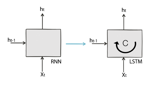
Long Short Term Memory network (LSTM)
\(h_t\) in RNN serves 2 purpose:
- Make an output prediction, and
- A hidden state representing the data sequence processed so far.
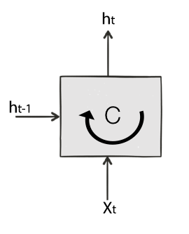
LSTM splits these 2 roles into 2 separate variables \(h_t\) and \(C\). The hidden state of the LSTM cell is now \(C\).
Here are the LSTM equations:
There are 3 gates controlling what information will pass through:
\[\begin{split} gate_{forget} &= \sigma (W_{fx} X_t + W_{fh} h_{t-1} + b_f) \\ gate_{input} &= \sigma (W_{ix} X_t + W_{ih} h_{t-1} + b_i) \\ gate_{out} &= \sigma (W_{ox} X_t + W_{oh} h_{t-1} + b_o) \\ \end{split}\]3 equations to update the cell state and the hidden state:
\[\begin{split} \tilde{C} & = \tanh (W_{cx} X_t + W_{ch} h_{t-1} + b_c) \\ C_t & = gate_{forget} \cdot C_{t-1} + gate_{input} \cdot \tilde{C} \\ h_t & = gate_{out} \cdot \tanh (C_t) \\ \end{split}\]Gates
There are 3 gates in LSTM. All gates are function of \(x_t\) and \(h_{t-1}\)
\[gate = \sigma (W_{x} X_t + W_{h} h_{t-1} + b) \\\]- \(gate_{forget}\) controls what part of the previous cell state will be kept.
- \(gate_{input}\) controls what part of the new computed information will be added to the cell state \(C\).
- \(gate_{out}\) controls what part of the cell state will exposed as the hidden state.
Updating C
The key part in LSTM is to update the cell state \(C\).
To do that, we need to compute a new proposal \(\tilde{C}\) just based in \(X_t\) and \(h_{t-1}\):
\[\tilde{C} = \tanh (W_{cx} X_t + W_{ch} h_{t-1} + b_c) \\\]The new state \(C_t\) is form by forgetting part of the previous cell state while add part of the new proposal \(\tilde{C}\) to the cell state:
\[\begin{split} C_t & = gate_{forget} \cdot C_{t-1} + gate_{input} \cdot \tilde{C} \\ \end{split}\]Update h
To update \(h_{t}\), we use the output gate to control what cell state to export as \(h_t\)
\[h_t = gate_{out} \cdot \tanh (C_t)\]Image captures with LSTM
Now we change our previous code and swap the RNN out with a LSTM.
if self.cell_type == 'rnn':
  h, cache_rnn = rnn_forward(x, h0, Wx, Wh, b)
else:
  h, cache_rnn = lstm_forward(x, h0, Wx, Wh, b)
lstm_forward looks similar to the RNN with the exception that it track both \(h\) and \(C\) now.
def lstm_forward(x, h0, Wx, Wh, b):
  h, cache = None, None
  N, T, D = x.shape
  H, _ = Wh.shape
  next_h = h0
  next_c = np.zeros((N, H))

  cache_step = [None] * T

  h = np.zeros((N, T, H))
  for t in range(T):
    xt = x[:, t, :]
    next_h, next_c, cache_step[t] = lstm_step_forward(xt, next_h, next_c, Wx, Wh, b)
    h[:, t, :] = next_h
  cache = (cache_step, D)

  return h, cache
One of the reason that we do not sub-index W and b is that we can concatenate all W and b into one big matrix and apply the matrix multiplication at once. The following code compute 3 different gates and then compute \(\tilde{C}\), \(C\) and \(h\) .
def lstm_step_forward(x, prev_h, prev_c, Wx, Wh, b):
  next_h, next_c, cache = None, None, None
  N, H = prev_h.shape
  a = x.dot(Wx) + prev_h.dot(Wh) + b
  ai = a[:, :H]
  af = a[:, H:2 * H]
  ao = a[:, 2 * H:3 * H]
  au = a[:, 3 * H:]
  ig = sigmoid(ai)
  fg = sigmoid(af)
  og = sigmoid(ao)
  update = np.tanh(au)
  next_c = fg * prev_c + ig * update
  next_h = og * np.tanh(next_c)

  cache = (next_c, og, ig, fg, og, update, ai, af, ao, au, Wx, x, Wh, prev_h, prev_c)

  return next_h, next_c, cache
LSTM composes of the Cell state and Hidden state. We use 3 gates to control what information will be passed through. We calculate new cell state by keep part of the original while adding new information. Then we expose part of the \(C_t\) as \(h_t\).
Gated Recurrent Units (GRU)
Compare with LSTM, GRU does not maintain a cell state \(C\) and use 2 gates instead of 3.
\[\begin{split} gate_r &= \sigma (W_{rx} X_t + W_{rh} h_{t-1} + b) \\ gate_{update} &= \sigma (W_{ux} X_t + W_{uh} h_{t-1} + b) \end{split}\]The new hidden state is compute as:
\[h_t = (1 - gate_{update}) \cdot h_{t-1} + gate_{update} \cdot \tilde{h_{t}}\]As seen, we use the compliment of \(gate_{update}\) instead of creating a new gate to control what we want to keep from the \(h_{t-1}\).
The new proposed \(\tilde{h_{t}}\) is calculated as:
\[\tilde{h_{t}} = \tanh (W_{hx} X_t + W_{hh} \cdot (gate_r \cdot h_{t-1}) + b)\]We use \(gate_r\) to control what part of \(h_{t-1}\) we need to compute a new proposal.
Credits
For the RNN/LSTM case study, we use the image caption assignment (assignment 3) in the Stanford class “CS231n Convolutional Neural Networks for Visual Recognition”. We start with the skeleton codes provided by the assignment and put it into our code to complete the assignment code.