“Soft & hard attention”
Generate image captions
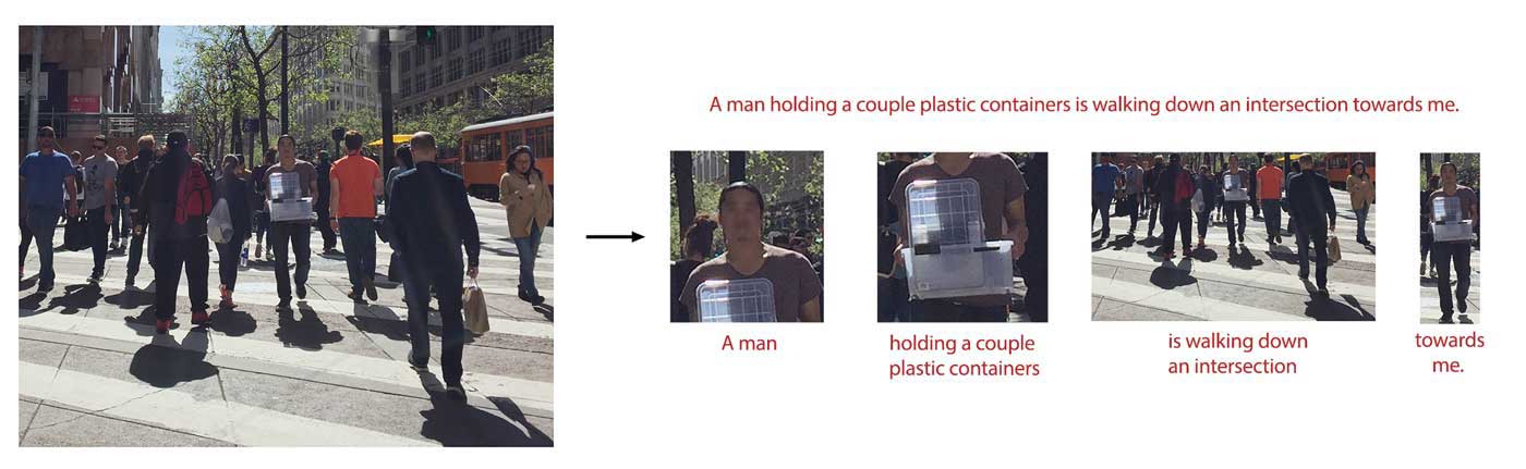
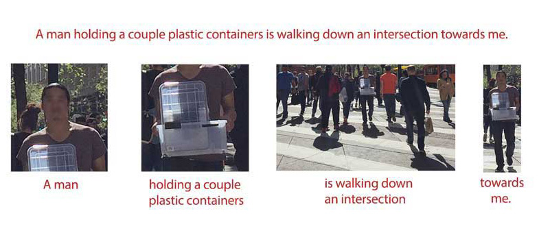
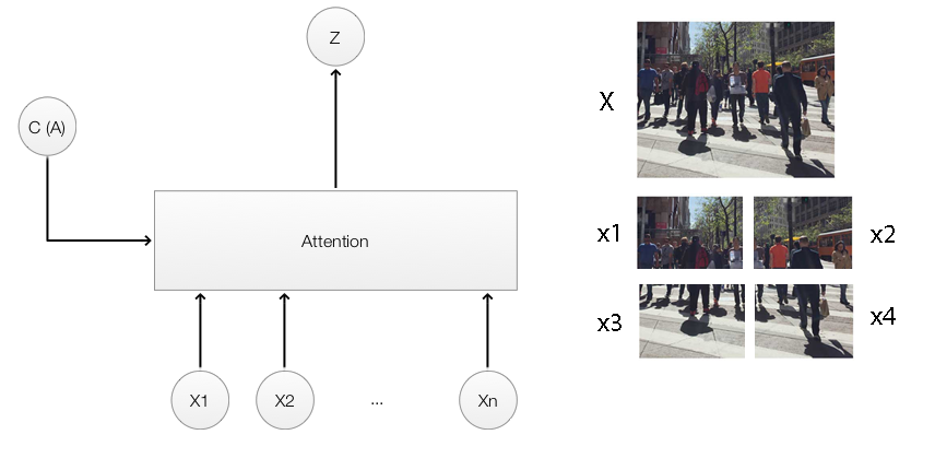
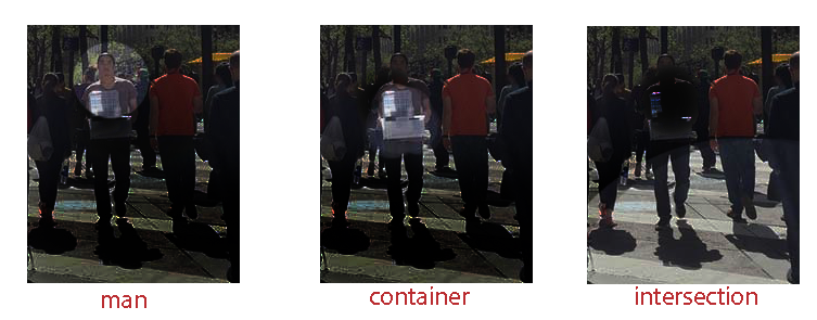
In cognitive science, selective attention illustrates how we restrict our attention to particular objects in the surroundings. It helps us focus, so we can tune out irrelevant information and concentrate on what really matters. We can apply this attention mechanism in solving many deep learning problems. For example, we focus on different areas of the image when generating an image caption. In the image below, we first pay attention to the closest man that walking towards us. We continue exploring the details or shift attentions according to the questions that we want to answer. Eventually, we may generate a caption like: “A man holding a couple plastic containers is walking down an intersection towards me.” Selective attention demonstrates objects or pixels are not treated equally. Attention in deep learning localizes information in making predictions. The picture below demonstrates the relationship between the attention area and the words we generate.
To generate an image caption with deep learning, we start the caption with a “start” token and generate one word at a time. We predict the next caption word based on the last predicted word and the image:
\[\text{next word} = f(image, \text{last word})\]Applying the RNN techniques, we rewrite the model as:
\[h_{t} = f(x, h_{t-1})\] \[\text{next word} = g(h_{t})\]which \(x\) is the image, and \(h_{t}\) is the RNN hidden state to predict the “next word” at time step \(t\).
We continue the process until we predict the “end” token. As the selective attention may suggest, this model is over-generalized, and we should replace the image with a more focus attention area.
\[h_{t} = f(attention(x, h_{t-1}), h_{t-1} )\]which \(attention\) generates features representing areas of focus from the image \(x\).
Image caption model with LSTM
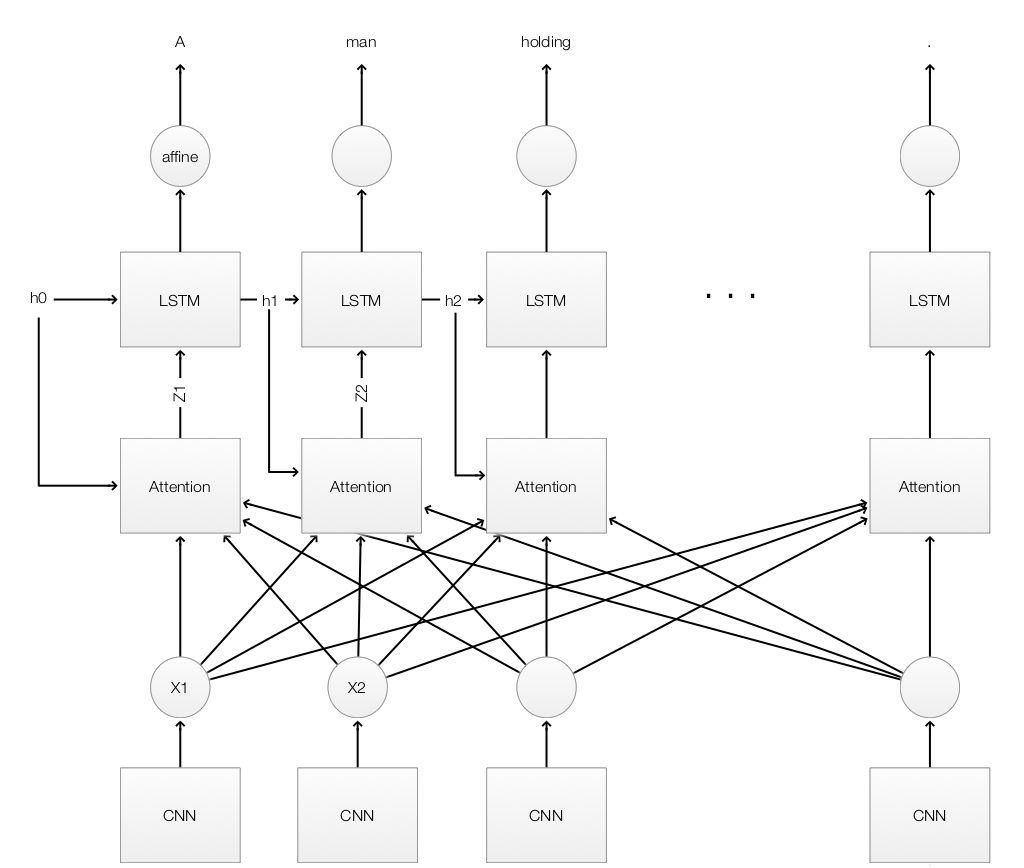
Before we discuss attention, we will have a quick review of the image caption using LSTM. We use a CNN to extract the features \(x\) from an image, and feed them to every LSTM cells. Each LSTM cell takes in the previous hidden state \(h_{t-1}\) and the image features \(x\) to calculate a new hidden state \(h_{t}\). We usually pass \(h_{t}\) to an affine operation to make a prediction on the next caption word \(y_{t}\).
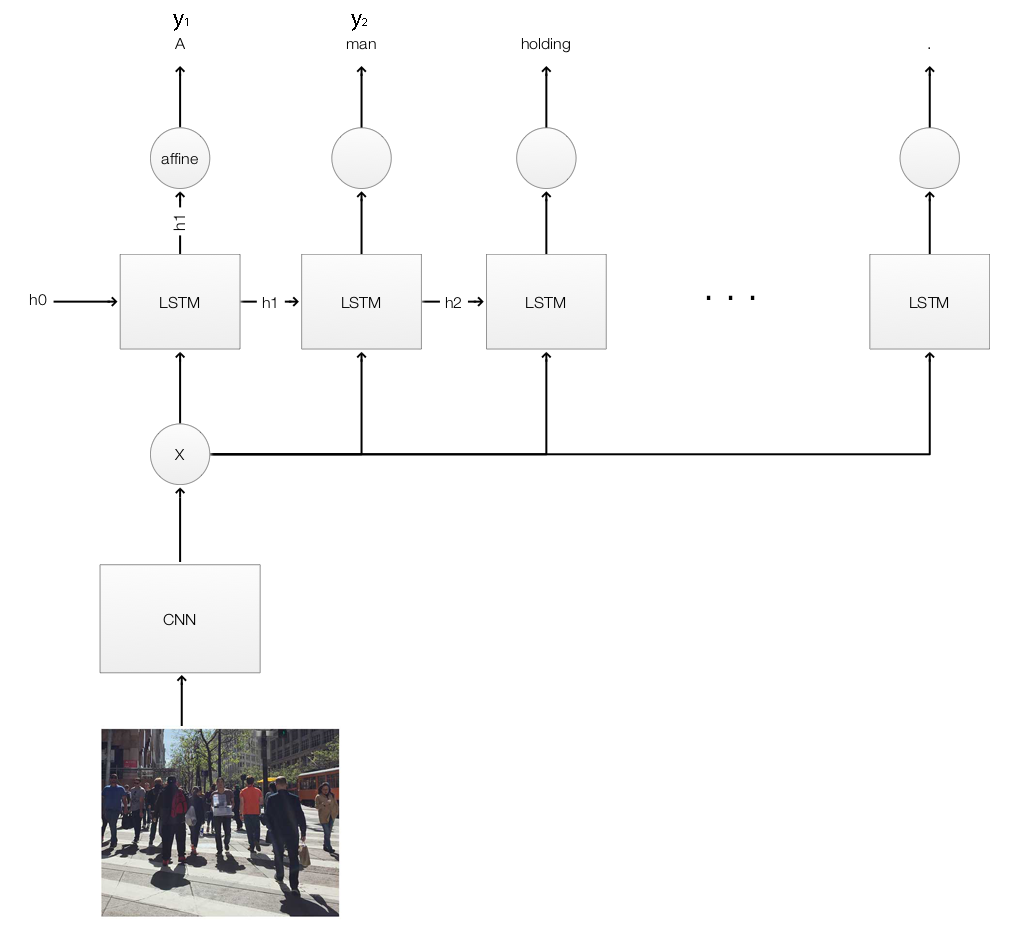
\(x\) are the image features extracted from an image using a CNN. From the LSTM perspective, \(x\) represents the image. When we reference the “image” in this article, we mean the image features \(x\) rather than the raw image pixels.
Attention
The key difference between a LSTM model and the one with attention is that “attention” pays attention to particular areas or objects rather than treating the whole image equally. For example, at the beginning of the caption creation, we start with an empty context. Our first attention area starts with the man who walks towards us. We predict the first word “A”, and update the context to “A”. We also keep the attention area unchanged. We make a second prediction “man” based on the context “A” and the attention area. For the next prediction, our attention shifts to what he is holding near his hand. By continue exploring or shifting the attention area and updating the context, we generate an caption like “ A man holding a couple plastic containers is walking down an intersection towards me.”
Mathematically, we are trying to replace the image \(x\) in LSTM model,
\[h_{t} = f(x, h_{t-1})\]with an attention module \(attention\):
\[h_{t} = f(attention(x, h_{t-1}), h_{t-1} )\]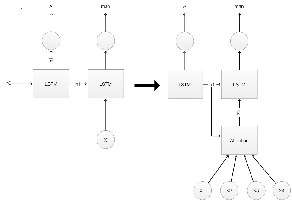
The attention module has 2 inputs:
- a context, and
- image features in each localized areas.
For the context, we use the hidden state \(h_{t-1}\) from the previous time step. In a LSTM system, we process an image with a CNN and use one of the fully connected layer output as input features \(x\) to the LSTM.
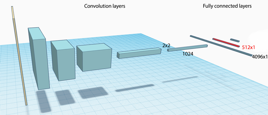
Nevertheless, this is not adequate for an attention model since spatial information has been lost. Instead, we use the feature maps of one of the convolution layer which spatial information is still preserved.
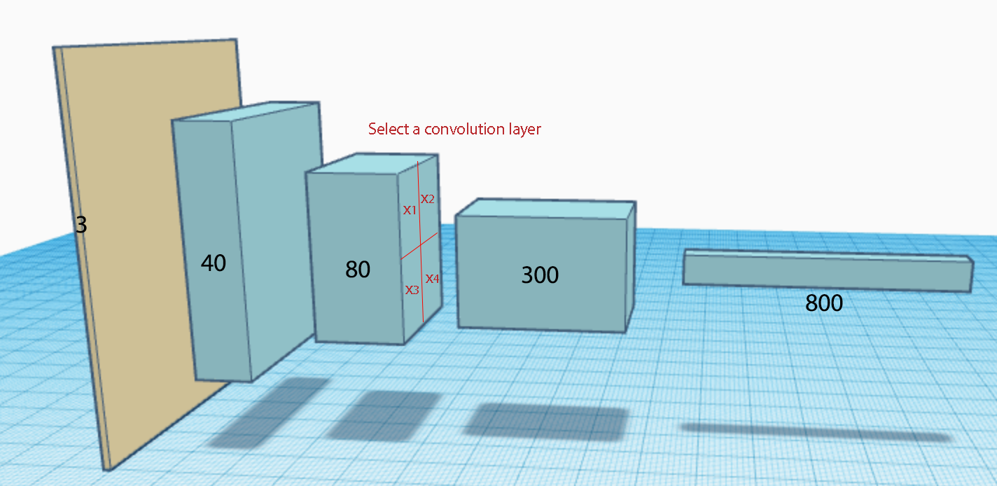
Here, the feature maps in the second convolution layers are divided into 4 which closely resemble the top right & left and the bottom right & left of the original pictures. We replace the LSTM input \(x\) with an attention module. The attention module takes the context \(h_{t-1}\) and 4 spatial regions \((x_1, x_2, x_3, x_{4})\) from the CNN to compute the new image features used by the LSTM.
\((x_1, x_2, x_3, x_{4})\) are features map. For demonstration purpose, we visualize the features maps in this article as the corresponding image that it may look like.
The following is the complete flow of the LSTM model using attentions.
Soft attention
We implement attention with soft attention or hard attention. In soft attention, instead of using the image \(x\) as an input to the LSTM, we input weighted image features accounted for attention. Before going into details, we can visualize the weighted features to illustrate the difference. Areas with higher attention are brighter in the picture.
Again, we visualize what the feature maps may look like as a picture.
This picture visualizes the weighted features to the LSTM and the word it predicted. Soft attention discredits irrelevant areas by multiply the corresponding features map with a low weight. Accordingly, high attention area keeps the original value while low attention areas get closer to 0 (become dark in the visualization). With the context of “A man holding a couple plastic”, the attention module creates a new feature map with all areas darkened except the plastic container area. With more focused information, the LSTM makes a better prediction (the word “container”).
Let’s show how to compute the weighted features for the LSTM. \(x_1, x_2, x_3 \text{ and } x_4\) each covers a sub-section of an image. To compute a score \(s_{i}\) to measure how much attention for \(x_{i}\), we use (with the context \(C = h_{t-1}\)):
\[s_{i} = \tanh(W_{c} C + W_{x} X_{i} ) = \tanh(W_{c} h_{t-1} + W_{x} x_{i} )\]We pass \(s_{i}\) to a softmax for normalization to compute the weight \(\alpha_{i}\).
\[\alpha_i = softmax(s_1, s_2, \dots, s_{i}, \dots)\]With softmax, \(\alpha_{i}\) adds up to 1, and we use it to compute a weighted average for \(x_1, x_2, x_3 \text{ and } x_4\)
\[Z = \sum_{i} \alpha_{i} x_{i}\]Finally, we use \(Z\) to replace \(x\) as the LSTM input.
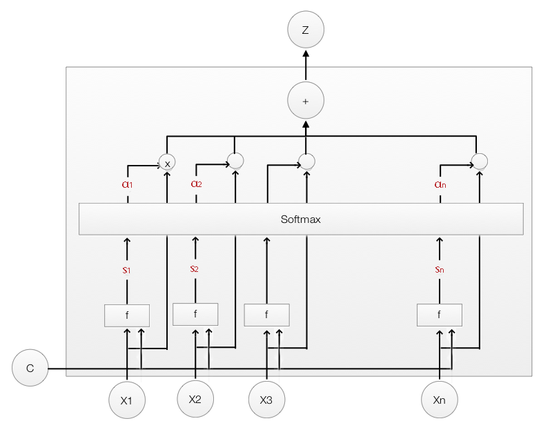
We compute scores \(\tanh(W_{c} h_{t-1} + W_{x} x_{i})\) for each area. Use the corresponding softmax values to computed a weighted input from the input features.
Hard attention
In soft attention, we compute a weight \(\alpha_{i}\) for each \(x_{i}\), and use it to calculate a weighted average for \(x_{i}\) as the LSTM input. \(\alpha_{i}\) adds up to 1 which can be interpreted as the probability that \(x_{i}\) is the area that we should pay attention to. So instead of a weighted average, hard attention uses \(\alpha_{i}\) as a sample rate to pick one \(x_{i}\) as the input to the LSTM.
\[Z \sim x_{i}, \alpha_{i}\]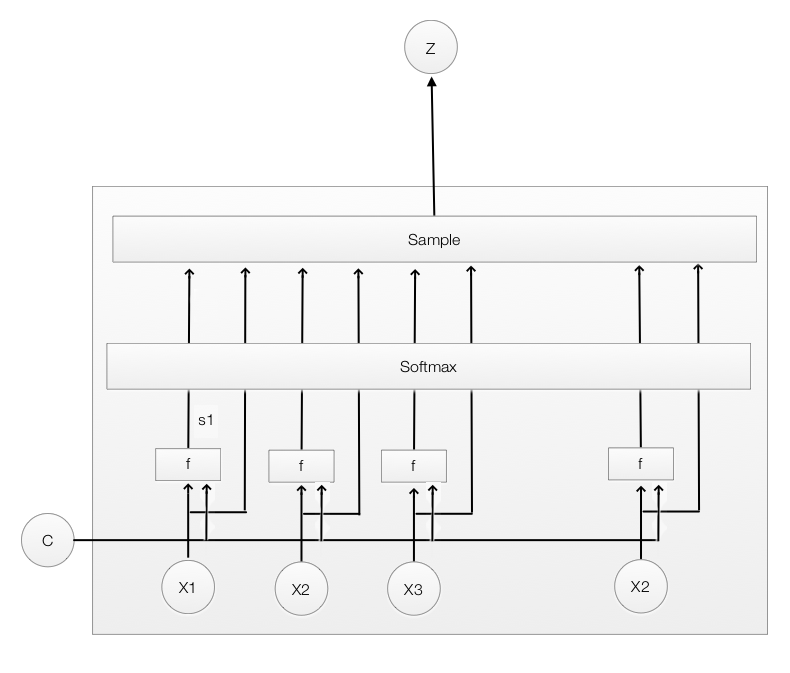
Hard attention replaces a deterministic method with a stochastic sampling model. To calculate the gradient descent correctly in the backpropagation, we perform samplings and average our results using the Monte Carlo method. Monte Carlo performs end-to-end episodes to compute an average for all sampling results. The accuracy is subject to how many samplings are performed and how well it is sampled. On the other hand, soft attention follows the regular and easier backpropagation method to compute the gradient. However, the accuracy is subject to the assumption that the weighted average is a good representation for the area of attention. Both have their shortcomings. Currently, soft attention is more popular.
Soft attention is more popular because the backpropagation seems more effective.