“Convolutional neural networks (CNN) tutorial”
Overview
In a fully connected network, all nodes in a layer are fully connected to all the nodes in the previous layer. This produces a complex model to explore all possible connections among nodes. But the complexity pays a high price in training the network and how deep the network can be. For spatial data like image, this complexity provides no additional benefits since most features are localized.
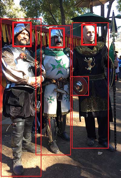
For face detection, the areas of interested are all localized. Convolution neural networks apply small size filter to explore the images. The number of trainable parameters is significantly smaller and therefore allow CNN to use many filters to extract interesting features.
Filters
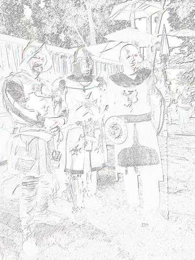
Filters are frequently applied to images for different purposes. The human visual system applies edge detection filters to recognize an object.
For example, to blur an image, we can apply a filter with patch size 3x3 over every pixel in the image:
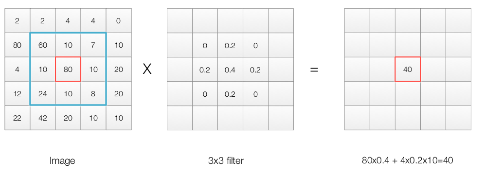
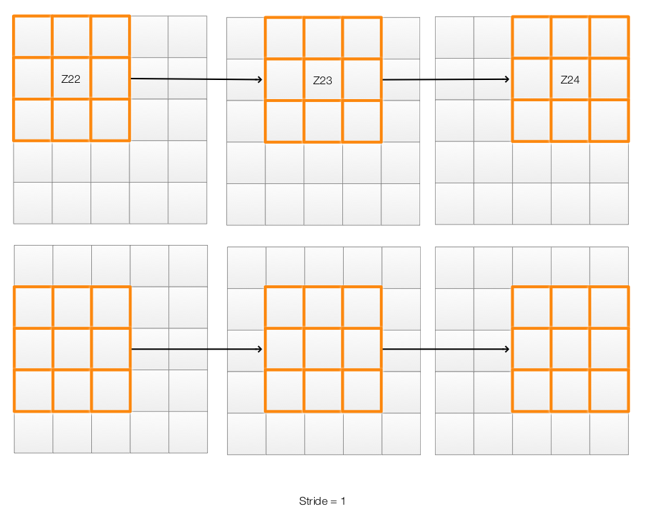
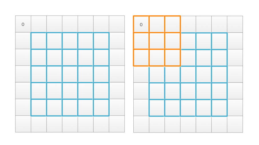
To apply the filter to an image, we move the filter 1 pixel at a time from left to right and top to bottom until we process every pixel.
Stride and padding
However, we may encounter some problem on the edge. For example, on the top left corner, a filter may cover beyond the edge of an image. For a filter with patch size 3x3, we may ignore the edge and generate an output with width and height reduce by 2 pixels. Otherwise, we can pack extra 0 or replicate the edge of the original image. All these settings are possible and configurable as “padding” in a CNN.
Padding with extra 0 is more popular because it maintains spatial dimensions and better preserve information on the edge.
For a CNN, sometimes we do not move the filter only by 1 pixel. If we move the filter 2 pixels to the right, we say the “X stride” is equal to 2.
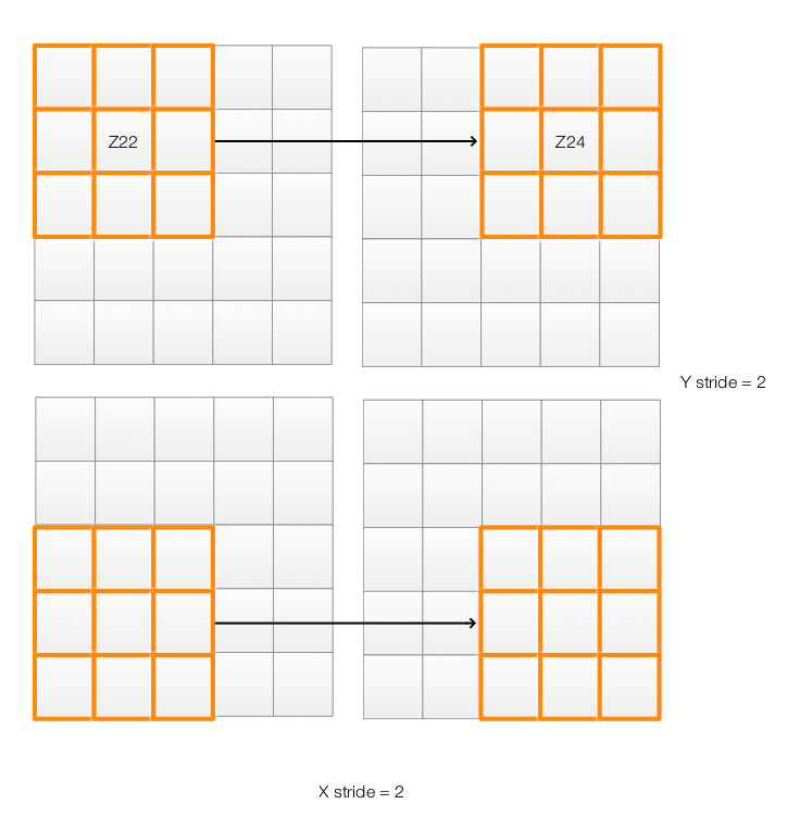
Notice that both padding and stride may change the spatial dimension of the output. A stride of 2 in X direction will reduce X-dimension by 2. Without padding and x stride equals 2, the output shrink N pixels:
\[N = \frac {\text{filter patch size} - 1} {2}\]Convolutional neural network (CNN)
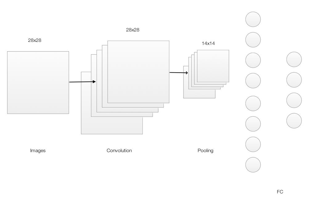
A convolutional neural network composes of convolution layers, polling layers and fully connected layers(FC).
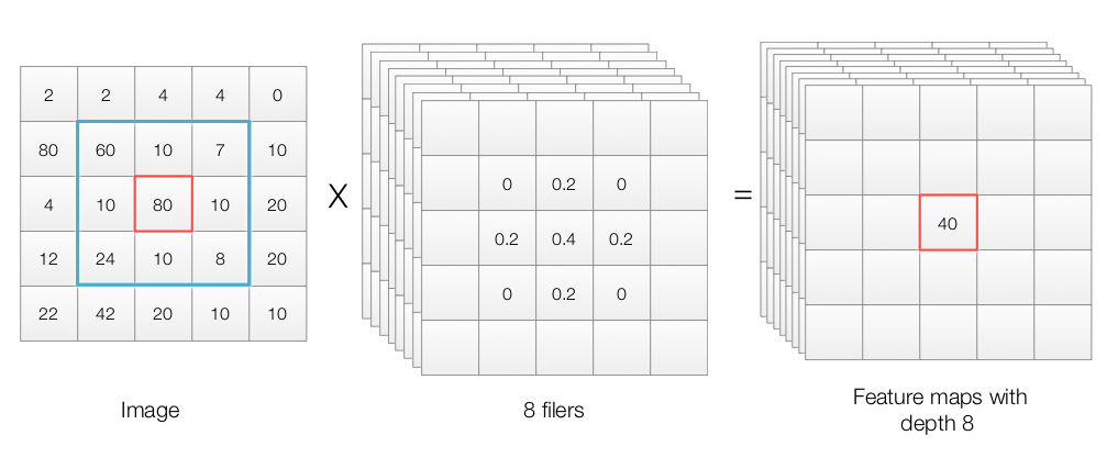
When we process the image, we apply filters which each generates an output that we call feature map. If k-features map is created, we have feature maps with depth k.
Visualization
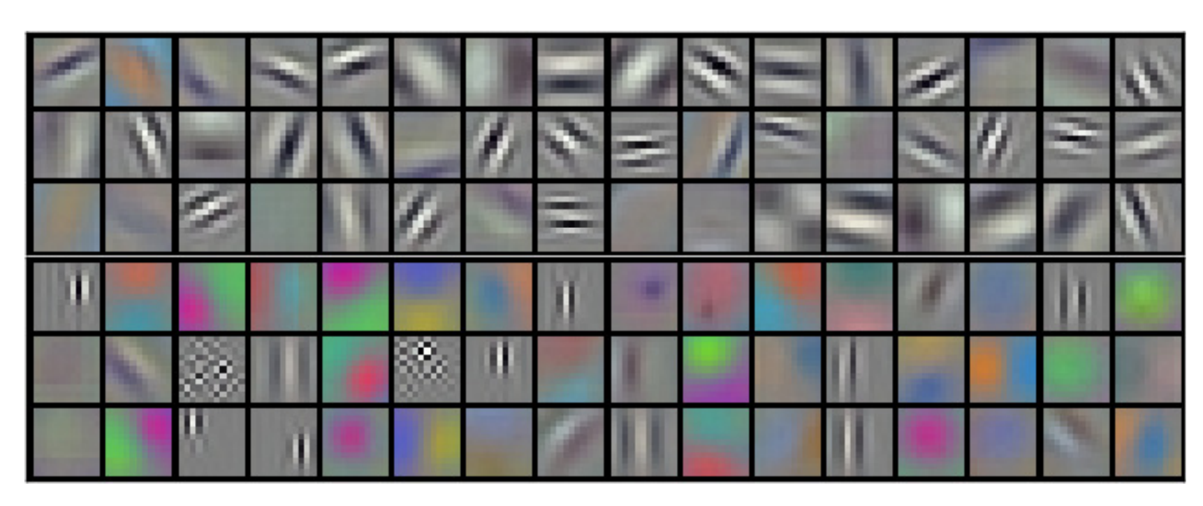
CNN uses filters to extract features of an image. It would be interesting to see what kind of filters that a CNN eventually trained. This gives us some insight understanding what the CNN trying to learn.
Here are the 96 filters learned in the first convolution layer in AlexNet. Many filters turn out to be edge detection filters common to human visual systems. (Source from Krizhevsky et al.)
The right side shows images with the highest activation in some feature maps at layer 4. Then we reconstruct the images based on the activations in the feature maps. This gives up some understanding of what the our model is looking for. (Source from Matthew D Zeiler et al.)
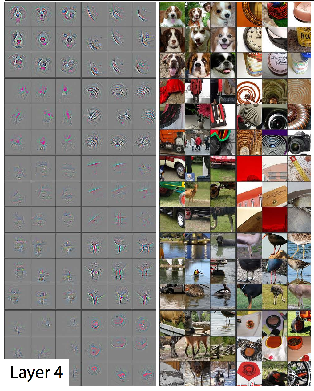
If the visualization of the filters seems lossy, it indicates we need more training iterations or we are overfitting.
Batch normalization & ReLU
After applying filters on the input, we apply a batch normalization followed by a ReLU for non-linearity. The batch normalization renormalizes data to make learning faster with the Gradient descent.
Batch normalization applies this equation to the input:
\[z = \frac{x - \mu}{\sigma}\]For a feature map with the spatial dimension 10x10, we compute 100 means and 100 variance from the batch samples. For example, if the batch size is 16, the mean for the feature at location (i, j) is computed by:
\[\mu_{i, j} = \frac{o^{(1)}_{i, j} + o^{(1)}_{i, j} + \dots + o^{(16)}_{i, j}}{16} \quad \text{which } o^{(k)} \text{ is the output from batch sample } k \in (1, 16)\\\]We feed \(z\) to a linear equation with the trainable scalar values \(\gamma\) and \(\beta\) (1 pair for each normalized layer).
\[out = \gamma z + \beta\]The normalization can be undone if \(gamma = \sigma\) and \(\beta = \mu\). We initialize \(\gamma = 1\) and \(\beta =0\), so the input is normalized and therefore learns faster, and the parameters will be learned during the training.
This is the code to implement batch normalization in TensorFlow:
w_bn = tf.Variable(w_initial)
z_bn = tf.matmul(x, w_bn)

bn_mean, bn_var = tf.nn.moments(z_bn, [0])
scale = tf.Variable(tf.ones([100]))
beta = tf.Variable(tf.zeros([100]))

bn_layer = tf.nn.batch_normalization(z_bn, bn_mean, bn_var, beta, scale, 1e-3)
l_bn = tf.nn.relu(bn_layer)
Pooling
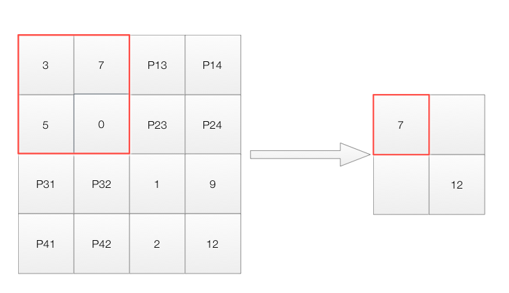
To reduce the spatial dimension of a feature map, we apply maximum pool. A 2x2 maximum pool replaces a 2x2 area by its maximum. After applying a 2x2 pool, we reduce the spatial dimension for the example below from 4x4 to 2x2. (Filter size=2, Stride = 2)
Here, we construct a CNN using convolution and pooling:
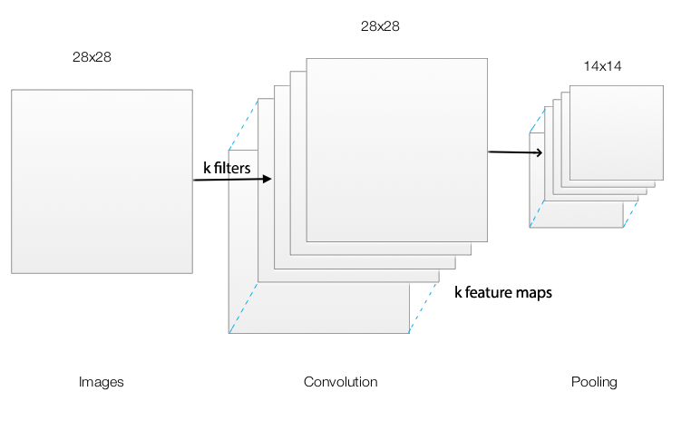
Pooling is often used with a convolution layer. Therefore, we often consider it as part of the convolution layer rather than a separate layer. The most common configuration is the maximum pool with filter size 2 and stride size 2. A filter size of 3 and stride size 2 is less common. Other pooling like average pooling has been used but fall out of favor lately. As a side note, some researcher may prefer using striding in a convolution filter to reduce dimension rather than pooling.
Multiple convolution layers
Like deep learning, the depth of the network increases the complexity of a model. A CNN network usually composes of many convolution layers.
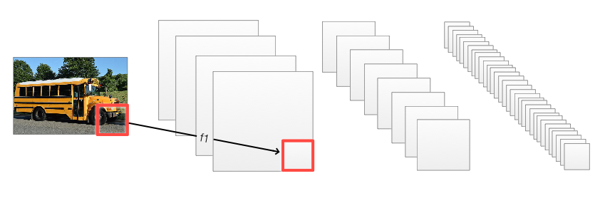
The CNN above composes of 3 convolution layer. We start with a 32x32 pixel image with 3 channels (RGB). We apply a 3x4 filter and a 2x2 max pooling which convert the image to 16x16x4 feature maps. The following table walks through the filter and layer shape at each layer:
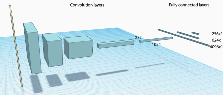
Fully connected (FC) layers
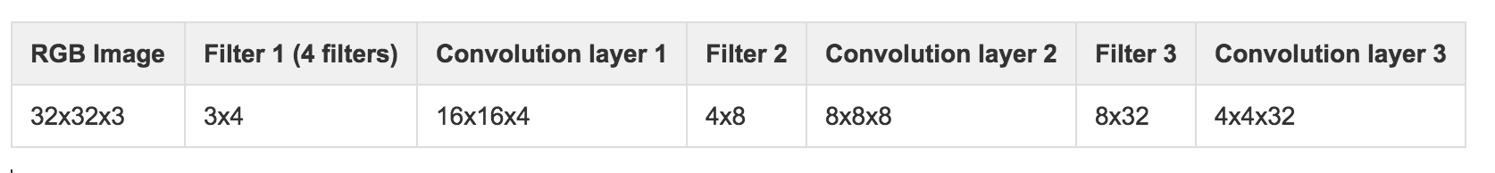
After using convolution layers to extract the spatial features of an image, we apply fully connected layers for the final classification. First, we flatten the output of the convolution layers. For example, if the final features maps have a dimension of 4x4x512, we will flatten it to an array of 8192 elements. We apply 2 more hidden layers here before we perform the final classification. The techniques needed are no difference from a FC network in deep learning.
Tips
Here are some of the tips to construct a CNN:
- Use smaller filters like 3x3 or 5x5 with more convolution layer.
- Convolution filter with small stride works better.
- If GPU memory is not large enough, sacrifice the first layer with a larger filter like 7x7 with stride 2.
- Use padding fill with 0.
- Use filter size 2, stride size 2 for the maximum pooling if needed.
For the network design:
- Start with 2-3 convolution layers with small filters 3x3 or 5x5 and no pooling.
- Add a 2x2 maximum pool to reduce the spatial dimension.
- Repeat 1-2 until a desired spatial dimension is reached for the fully connected layer. This can be a try and error process.
- Use 2-3 hidden layers for the fully-connection layers.
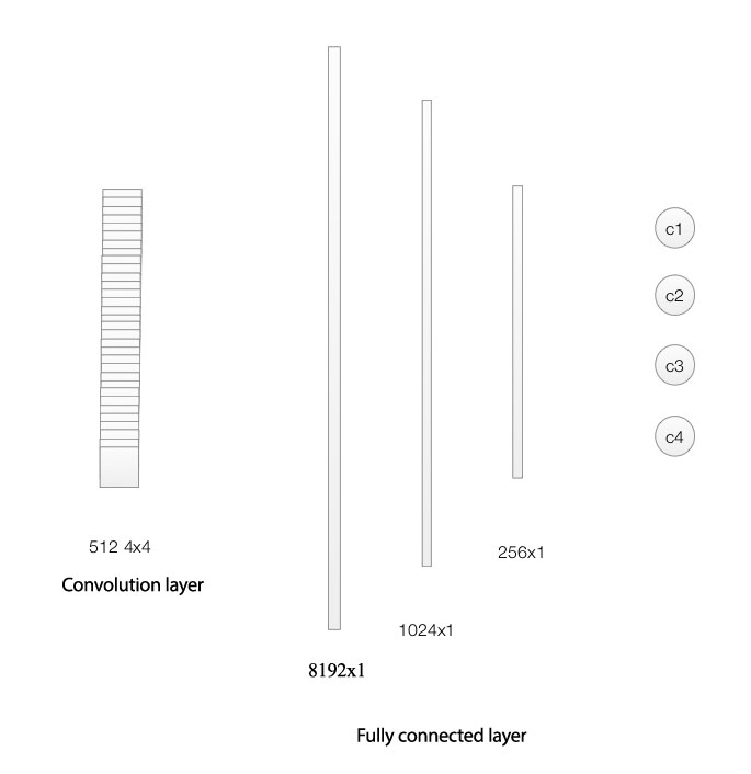
Convolutional pyramid
For each convolution layer, we reduce the spatial dimension while increasing the depth of the feature maps. Because of the shape, we call this a convolutional pyramid.
Here, we reduce the spatial dimension of each convolution layer through pooling or sometimes apply a filter with stride size > 1.
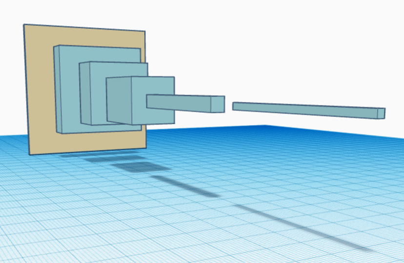
The depth of the feature map can be increased by applying more filters.
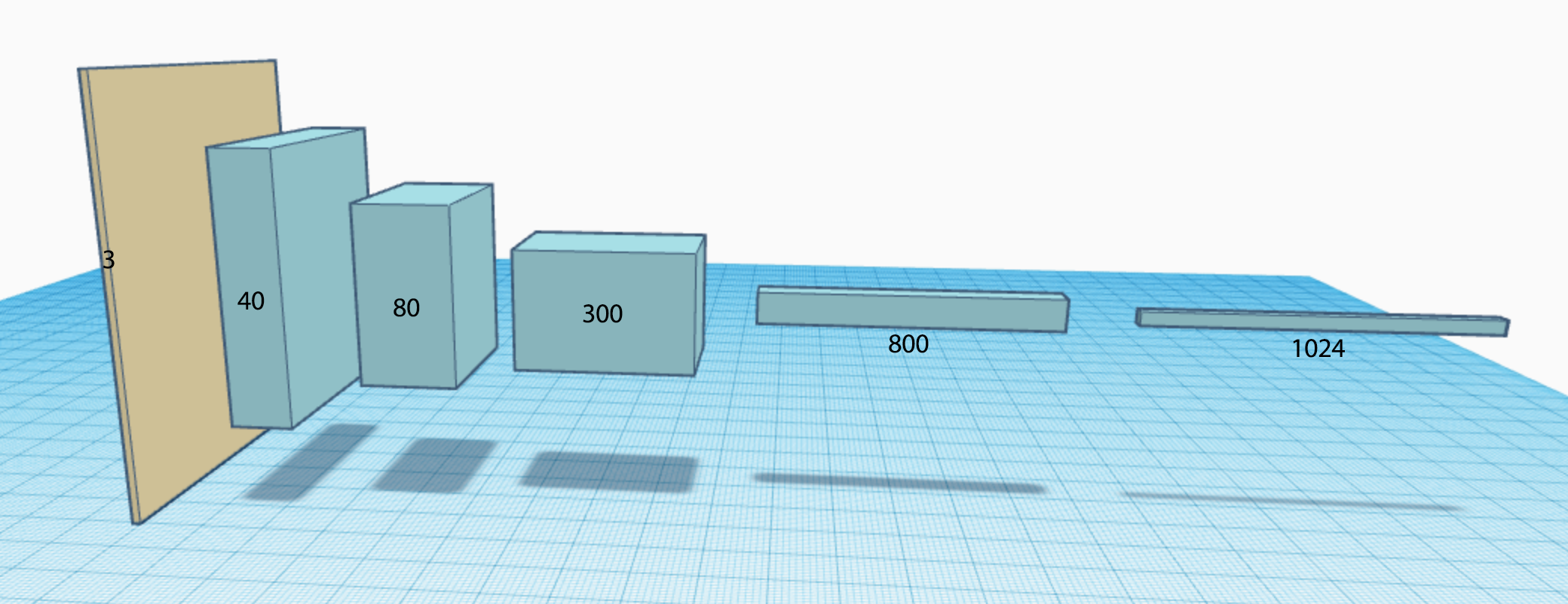
The core thinking of CNN is to apply small filters to explore spatial feature. The spatial dimension will gradually decrease as we go deep into the network. On the other hand, the depth of the feature maps will increase. It will eventually reach a stage that spatial locality is less important and we can apply a FC network for final analysis.
Google inceptions with 1x1 convolution
In our previous discussion, the convolution filter in each layer is of the same patch size say 3x3. To increase the depth of the feature maps, we can apply more filters using the same patch size. However, in GoogleNet, it applies a different approach to increase the depth. GoogleNet uses different filter patch size for the same layer. Here we can have filters with patch size 3x3 and 1x1. Don’t mistake that a 1x1 filter is doing nothing. It does not explore the spatial dimension but it explores the depth of the feature maps. For example, in the 1x1 filter below, we convert the RGB channels (depth 3) into two feature maps output. The first set of filters generates 8 features map while the second one generates two. We can concatenate them to form maps of depth 10. The inception idea is to increase the depth of the feature map by concatenating feature maps using different patch size of convolution filters and pooling.
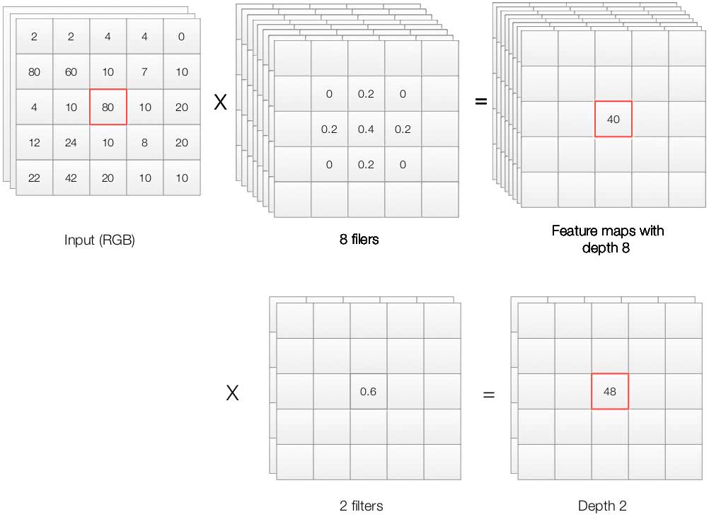
Inceptions can be considered as one way to introduce non-linearity into the system.
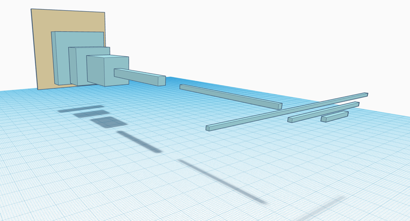
Fully connected network
After exploring the spatial relationship, we flatten the convolution layer output and connect it to a fully connected network:
TensoFlowr code
We will implement coding for a CNN to classify handwriting for digits (0 to 9).
We will use TensorFlow to implement a CNN. Nevertheless, the full understanding of the code is not needed or suggested even the code is pretty self-explainable.
Construct a CNN
In the code below, we construct a CNN with 2 convolution layer followed by 2 FC layer and then 1 classifier. Here is where we construct our CNN network.
# Model.
def model(data):
    # First convolution layer with stride = 1 and pad the edge to make the output size the same.
    # Apply ReLU and a maximum 2x2 pool
    conv1 = tf.nn.conv2d(data, cnn1_W, [1, 1, 1, 1], padding='SAME')
    hidden1 = tf.nn.relu(conv1 + cnn1_b)
    pool1 = tf.nn.max_pool(hidden1, [1, 2, 2, 1], [1, 2, 2, 1], padding='SAME')

    # Second convolution layer
    conv2 = tf.nn.conv2d(pool1, cnn2_W, [1, 1, 1, 1], padding='SAME')
    hidden2 = tf.nn.relu(conv2 + cnn2_b)
    pool2 = tf.nn.max_pool(hidden2, [1, 2, 2, 1], [1, 2, 2, 1], padding='SAME')

    # Flattern the convolution output
    shape = pool2.get_shape().as_list()
    reshape = tf.reshape(pool2, [shape[0], shape[1] * shape[2] * shape[3]])

    # 2 FC hidden layers
    fc1 = tf.nn.relu(tf.matmul(reshape, fc1_W) + fc1_b)
    fc2 = tf.nn.relu(tf.matmul(fc1, fc2_W) + fc2_b)

    # Return the result of the classifier
    return tf.matmul(fc2, classifier_W) + classifier_b
For the convolution filter, we want the output spatial dimension to be the same as the input and therefore we assign padding = “same”. We also have stride = 1. After the filter, we apply the standard ReLU and a 2x2 maximum pool.
conv1 = tf.nn.conv2d(data, cnn1_W, [1, 1, 1, 1], padding='SAME')
hidden1 = tf.nn.relu(conv1 + cnn1_b)
pool1 = tf.nn.max_pool(hidden1, [1, 2, 2, 1], [1, 2, 2, 1], padding='SAME')
After the second convolution layer, we flatten the layer for the FC layer.
shape = pool2.get_shape().as_list()
reshape = tf.reshape(pool2, [shape[0], shape[1] * shape[2] * shape[3]])
We applied 2 FC layers before return the result from the classifier.
fc1 = tf.nn.relu(tf.matmul(reshape, fc1_W) + fc1_b)
fc2 = tf.nn.relu(tf.matmul(fc1, fc2_W) + fc2_b)

# Return the result of the classifier
return tf.matmul(fc2, classifier_W) + classifier_b
CNN configuration:
Here is our model configuration. We have 2 Convolution layers both using a filter with patch size 5x5 and generate feature maps with depth 16. The first FC output 256 values while the second output 64.
batch_size = 16
patch_size = 5
depth = 16
num_hidden1 = 256
num_hidden2 = 64
Here is where we define the trainable parameters for CNN layer 1 and 2. For example, the shape of the weight in cnn1 is 5x5x3x16. It applies 5x5 filter patch for RGB channels which output feature maps with depth 16.
# CNN layer 1 with filter (num_channels, depth) (3, 16)
cnn1_W = tf.Variable(tf.truncated_normal([patch_size, patch_size, num_channels, depth], stddev=0.1))
cnn1_b = tf.Variable(tf.zeros([depth]))

# CNN layer 2 with filter (depth, depth) (16, 16)
cnn2_W = tf.Variable(tf.truncated_normal([patch_size, patch_size, depth, depth], stddev=0.1))
cnn2_b = tf.Variable(tf.constant(1.0, shape=[depth]))
Here are the FC trainable parameters that is not much difference from other deep learning network using FC.
 # Compute the output size of the CNN2 as a 1D array.
size = image_size // 4 * image_size // 4 * depth

# FC1 (size, num_hidden1) (size, 256)
fc1_W = tf.Variable(tf.truncated_normal([size, num_hidden1], stddev=np.sqrt(2.0 / size)))
fc1_b = tf.Variable(tf.constant(1.0, shape=[num_hidden1]))

# FC2 (num_hidden1, num_hidden2) (size, 64)
fc2_W = tf.Variable(tf.truncated_normal([num_hidden1, num_hidden2], stddev=np.sqrt(2.0 / (num_hidden1))))
fc2_b = tf.Variable(tf.constant(1.0, shape=[num_hidden2]))

# Classifier (num_hidden2, num_labels) (64, 10)
classifier_W = tf.Variable(tf.truncated_normal([num_hidden2, num_labels], stddev=np.sqrt(2.0 / (num_hidden2))))
classifier_b = tf.Variable(tf.constant(1.0, shape=[num_labels]))
Here is the full code for completeness. Nevertheless, the code requires the datafile ‘notMNIST.pickle’ to run which is not provided here.
import matplotlib.pyplot as plt
import numpy as np
import tensorflow as tf
import pickle
import os


def set_working_dir():
    tmp_dir = 'tmp'
    if not os.path.exists(tmp_dir):
        os.makedirs(tmp_dir)
    os.chdir(tmp_dir)
    print("Change working directory to", os.getcwd())


set_working_dir()

pickle_file = 'notMNIST.pickle'

with open(pickle_file, 'rb') as f:
    save = pickle.load(f)
    train_dataset = save['train_dataset']
    train_labels = save['train_labels']
    valid_dataset = save['valid_dataset']
    valid_labels = save['valid_labels']
    test_dataset = save['test_dataset']
    test_labels = save['test_labels']
    del save  # hint to help gc free up memory
    print('Training set', train_dataset.shape, train_labels.shape)
    print('Validation set', valid_dataset.shape, valid_labels.shape)
    print('Test set', test_dataset.shape, test_labels.shape)

image_size = 28
num_labels = 10
num_channels = 1 # grayscale


def reformat(dataset, labels):
  dataset = dataset.reshape(
    (-1, image_size, image_size, num_channels)).astype(np.float32)
  labels = (np.arange(num_labels) == labels[:,None]).astype(np.float32)
  return dataset, labels
train_dataset, train_labels = reformat(train_dataset, train_labels)
valid_dataset, valid_labels = reformat(valid_dataset, valid_labels)
test_dataset, test_labels = reformat(test_dataset, test_labels)
print('Training set', train_dataset.shape, train_labels.shape)
print('Validation set', valid_dataset.shape, valid_labels.shape)
print('Test set', test_dataset.shape, test_labels.shape)


def accuracy(predictions, labels):
  return (100.0 * np.sum(np.argmax(predictions, 1) == np.argmax(labels, 1))
          / predictions.shape[0])

batch_size = 16
patch_size = 5
depth = 16
num_hidden1 = 256
num_hidden2 = 64

graph = tf.Graph()

with graph.as_default():
    # Define the training dataset and lables
    tf_train_dataset = tf.placeholder(
        tf.float32, shape=(batch_size, image_size, image_size, num_channels))
    tf_train_labels = tf.placeholder(tf.float32, shape=(batch_size, num_labels))

    # Validation/test dataset
    tf_valid_dataset = tf.constant(valid_dataset)
    tf_test_dataset = tf.constant(test_dataset)

    # CNN layer 1 with filter (num_channels, depth) (3, 16)
    cnn1_W = tf.Variable(tf.truncated_normal(
        [patch_size, patch_size, num_channels, depth], stddev=0.1))
    cnn1_b = tf.Variable(tf.zeros([depth]))

    # CNN layer 2 with filter (depth, depth) (16, 16)
    cnn2_W = tf.Variable(tf.truncated_normal(
        [patch_size, patch_size, depth, depth], stddev=0.1))
    cnn2_b = tf.Variable(tf.constant(1.0, shape=[depth]))

    # Compute the output size of the CNN2 as a 1D array.
    size = image_size // 4 * image_size // 4 * depth

    # FC1 (size, num_hidden1) (size, 256)
    fc1_W = tf.Variable(tf.truncated_normal(
        [size, num_hidden1], stddev=np.sqrt(2.0 / size)))
    fc1_b = tf.Variable(tf.constant(1.0, shape=[num_hidden1]))

    # FC2 (num_hidden1, num_hidden2) (size, 64)
    fc2_W = tf.Variable(tf.truncated_normal(
        [num_hidden1, num_hidden2], stddev=np.sqrt(2.0 / (num_hidden1))))
    fc2_b = tf.Variable(tf.constant(1.0, shape=[num_hidden2]))

    # Classifier (num_hidden2, num_labels) (64, 10)
    classifier_W = tf.Variable(tf.truncated_normal(
        [num_hidden2, num_labels], stddev=np.sqrt(2.0 / (num_hidden2))))
    classifier_b = tf.Variable(tf.constant(1.0, shape=[num_labels]))

    # Model.
    def model(data):
        # First convolution layer with stride = 1 and pad the edge to make the output size the same.
        # Apply ReLU and a maximum 2x2 pool
        conv1 = tf.nn.conv2d(data, cnn1_W, [1, 1, 1, 1], padding='SAME')
        hidden1 = tf.nn.relu(conv1 + cnn1_b)
        pool1 = tf.nn.max_pool(hidden1, [1, 2, 2, 1], [1, 2, 2, 1], padding='SAME')

        # Second convolution layer
        conv2 = tf.nn.conv2d(pool1, cnn2_W, [1, 1, 1, 1], padding='SAME')
        hidden2 = tf.nn.relu(conv2 + cnn2_b)
        pool2 = tf.nn.max_pool(hidden2, [1, 2, 2, 1], [1, 2, 2, 1], padding='SAME')

        # Flattern the convolution output
        shape = pool2.get_shape().as_list()
        reshape = tf.reshape(pool2, [shape[0], shape[1] * shape[2] * shape[3]])

        # 2 FC hidden layers
        fc1 = tf.nn.relu(tf.matmul(reshape, fc1_W) + fc1_b)
        fc2 = tf.nn.relu(tf.matmul(fc1, fc2_W) + fc2_b)

        # Return the result of the classifier
        return tf.matmul(fc2, classifier_W) + classifier_b

    # Training computation.
    logits = model(tf_train_dataset, True)
    loss = tf.reduce_mean(
        tf.nn.softmax_cross_entropy_with_logits(labels=tf_train_labels, logits=logits))

    # Optimizer.
    optimizer = tf.train.AdamOptimizer(0.0005).minimize(loss)

    # Predictions for the training, validation, and test data.
    train_prediction = tf.nn.softmax(logits)
    valid_prediction = tf.nn.softmax(model(tf_valid_dataset))
    test_prediction = tf.nn.softmax(model(tf_test_dataset))

num_steps = 20001

with tf.Session(graph=graph) as session:
  tf.global_variables_initializer().run()
  print('Initialized')
  for step in range(num_steps):
    offset = (step * batch_size) % (train_labels.shape[0] - batch_size)
    batch_data = train_dataset[offset:(offset + batch_size), :, :, :]
    batch_labels = train_labels[offset:(offset + batch_size), :]
    feed_dict = {tf_train_dataset : batch_data, tf_train_labels : batch_labels}
    _, l, predictions = session.run(
      [optimizer, loss, train_prediction], feed_dict=feed_dict)
    if (step % 500 == 0):
      print('Minibatch loss at step %d: %f' % (step, l))
      print('Minibatch accuracy: %.1f%%' % accuracy(predictions, batch_labels))
      print('Validation accuracy: %.1f%%' % accuracy(
        valid_prediction.eval(), valid_labels))
  print('Test accuracy: %.1f%%' % accuracy(test_prediction.eval(), test_labels))

  # Test accuracy: 95.2%
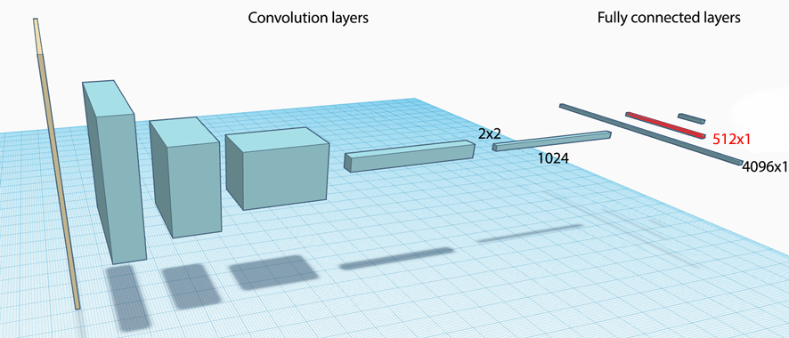
Transfer learning
Training a network can take a long time and a large dataset. Transfer learning is about using other people models to solve your problems. For example, can we use a pre-built natural language processing network in English for Spanish? Can we use a CNN network to predict different kinds of classes? In practice, there are more commons than we think. The features extracted at earlier layers are similar in many problem domains. For example, we can reuse a mature CNN model pre-trained with a huge dataset, and replace a few right most FC layers. In the network below, we replace the red layer and the ones on its right. We can add or remove nodes and layers. We initialize these new layers and train with our smaller dataset. There are 2 options in the training. Allow the whole system to be trained or just perform gradient descent on the changed layers.
In addition, we can feed the activation output at certain layer to a different network to solve a different problem. For example, we want to create a caption for images automatically. First, we can process images by a CNN and use the features in the FC layer as input to a recurrent network to generate caption.
Credits
For the TensorFlow coding, we start with the CNN class assignment 4 from the Google deep learning class on Udacity. We implement a CNN design with additional code to complete the assignment.