“Understanding Dynamic Routing between Capsules (Capsule Networks)”
This article covers the technical paper by Sara Sabour, Nicholas Frosst and Geoffrey Hinton on Dynamic Routing between Capsules. In this article, we will describe the basic Capsule concept and apply it with the Capsule network CapsNet to detect digits in MNist. In the last third of the article, we go through a detail implementation. The source code implementation is originated from XifengGuo using Keras with Tensorflow.
CNN challenges
In deep learning, the activation level of a neuron is often interpreted as the likelihood of detecting a specific feature.
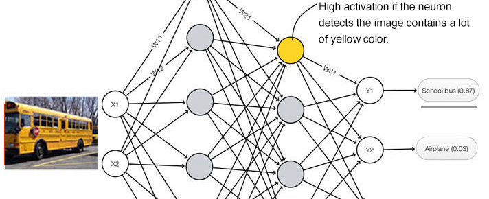
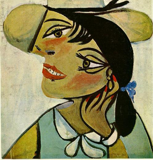
If we pass the Picasso’s “Portrait of woman in d`hermine pass” into a CNN classifier, how likely that the classifier may mistaken it as a real human face?
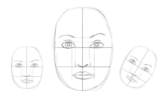
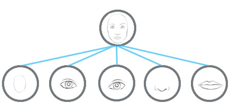
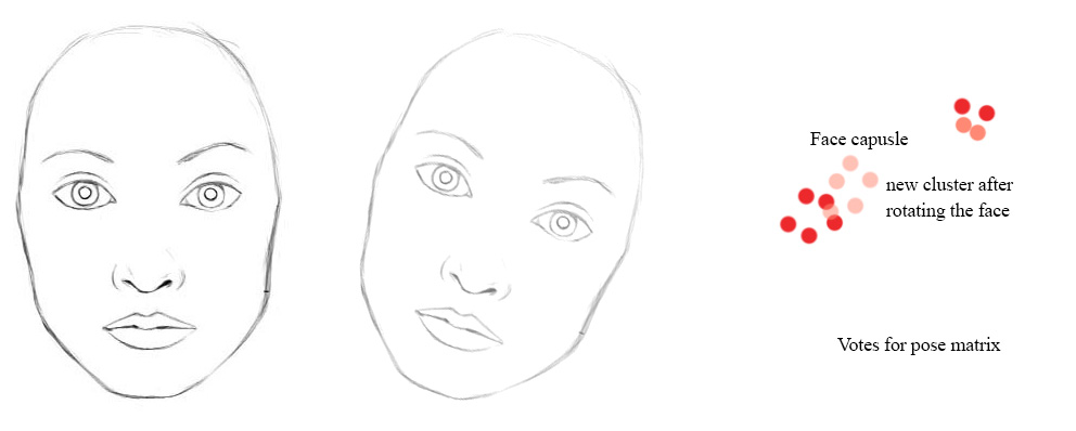
CNN is good at detecting features but less effective at exploring the spatial relationships among features (perspective, size, orientation). For example, the following picture may fool a simple CNN model in believing that this a good sketch of a human face.
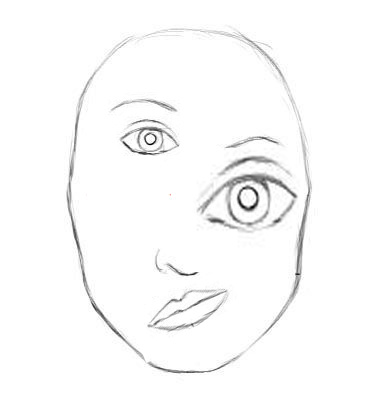
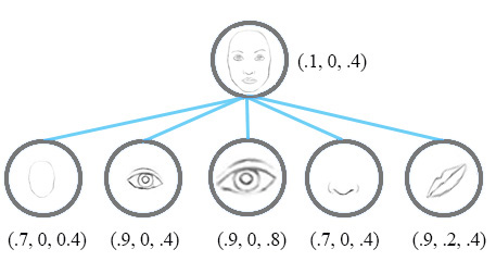
A simple CNN model can extract the features for nose, eyes and mouth correctly but will wrongly activate the neuron for the face detection. Without realize the mis-match in spatial orientation and size, the activation for the face detection will be too high.
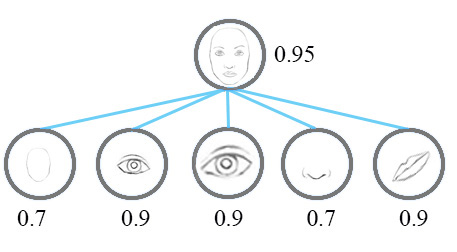
Now, we imagine that each neuron contains the likelihood as well as properties of the features. For example, it outputs a vector containing [likelihood, orientation, size]. With this spatial information, we can detect the in-consistence in the orientation and size among the nose, eyes and ear features and therefore output a much lower activation for the face detection.
Instead of using the term neurons, the technical paper uses the term capsules to indicate that capsules output a vector instead of a single scaler value.
Equivariance
Conceptually, a CNN model uses multiple neurons and layers in capturing different feature’s variants:
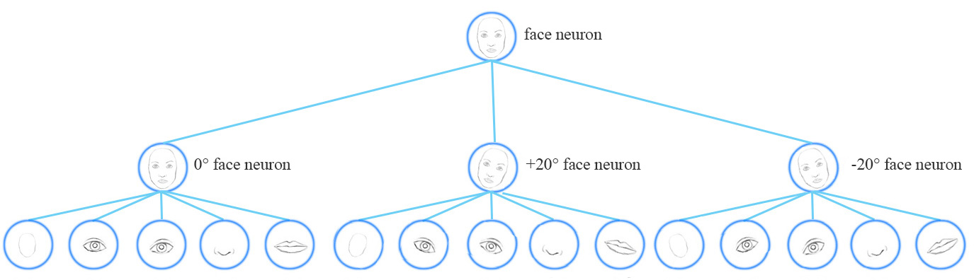
A capsule network share the same capsule to detect multiple variants in a simpler network.
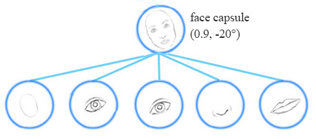
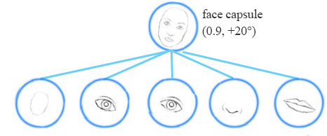
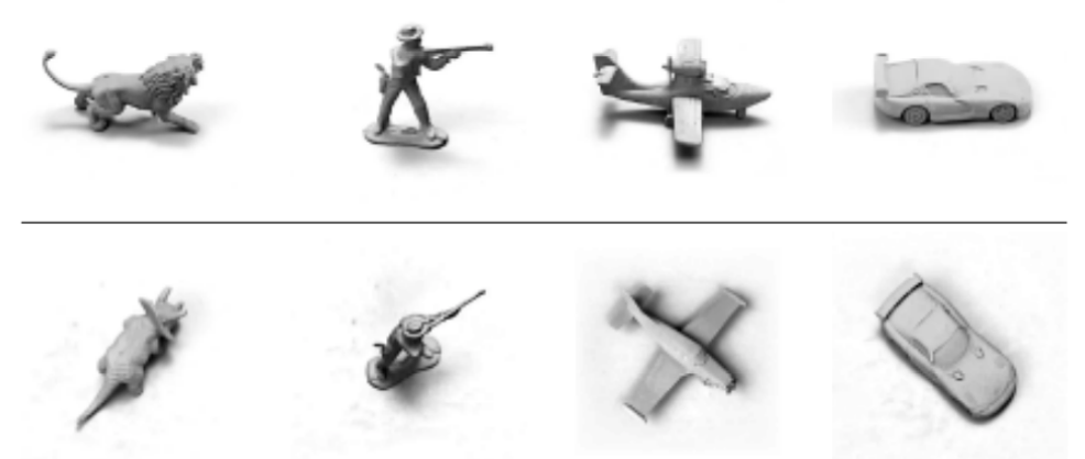
Equivariance is the detection of objects that can transform to each other. Intuitively, a capsule detects the face is rotated right 20° (or rotated left 20°) rather than realizes the face matched a variant that is rotated right 20°. By forcing the model to learn the feature variant in a capsule, we may extrapolate possible variants more effectively with less training data.
MNist dataset contains 55,000 training data. i.e. 5,500 samples per digits. However, it is unlikely that children need to read this large amount of samples to learn digits. Our existing deep learning models including CNN seem inefficient in utilizing datapoints.
With feature property as part of the information extracted by capsules, we may generalize the model better without an over extensive amount of labeled data.
Capsule
A capsule is a group of neurons that not only capture the likelihood but also the parameters of the specific feature.
For example, the first row below indicates the probabilities of detecting the number “7” by a neuron. A 2-D capsule is formed by combining 2 neurons. This capsule outputs a 2-D vector in detecting the number “7”. For the first image in the second row, it outputs a vector \(v = (0, 0.9)\). The magnitude of the vector \(\| v \| = \sqrt{ 0^2 + 0.9^2 } = 0.9\) corresponds to the probability of detecting “7”. The second image of each row looks more like a “1” than a “7”. Therefore its corresponding likelihood as “7” is smaller (smaller scaler value or smaller vector’s magnitude but with the same orientation) .
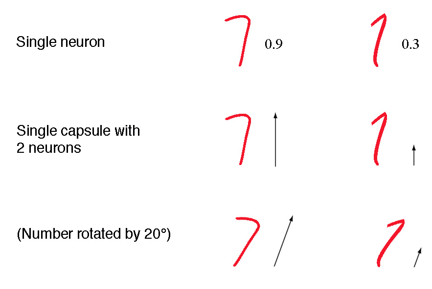
In the third row, we rotate the image by 20°. The capsule will generate vectors with the same magnitude but different orientations. Here, the angle of the vector represents the angle of rotation for the number “7”. As we can image, we can add 2 more neurons to a capsule to capture the size and stroke width.
We call the output vector of a capsule as the activity vector with magnitude represents the probability of detecting a feature and its orientation represents its parameters (properties).
Dynamic routing
Dynamic routing groups capsules to form a parent capsule, and it calculates the capsule’s output.
Intuition
We collect 3 similar sketches with different scale and orientation, and we measures the horizontal width of the mouth and the eye in pixels. They are \(s^{(1)}=(100, 66), s^{(2)}=(200, 131) \text{ and } s^{(3)}=( 50, 33).\)
Let’s assume \(W_m =2, W_e=3\), and we calculate a vote from the mouth and the eye for \(s^{(1)}\) as:
\[\begin{split} v^{(1)}_m & = W_m \times width_m = 2 \times 100 = 200 \\ v^{(1)}_e & = W_e \times width_e = 3 \times 66 = 198 \\ \end{split}\]We realize both \(v^{(1)}_m\) and \(v^{(1)}_e\) are very similar. When we repeat it with other sketches, we get the same findings. So the mouth capsule and the eye capsule can be strongly related to a parent capsule with width approximate 200 pixels. From our experience, a face is 2 times (\(W_m=2\)) the width of a mouth and 3 times the width (\(W_e=3\)) of an eye. So the parent capsule we detected is a face capsule. Of course, we can make it more accurate by adding more properties like height or color. In dynamic routing, we transform the vectors of an input capsules with a transformation matrix \(W\) to form a vote, and group capsules with similar votes. Those votes eventually becomes the output vector of the parent capsule. So how can we know \(W\)? Just do it in the deep learning way: backpropagation with a cost function.
Calculating a capsule output
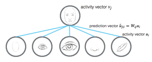
For a capsule, the input \(u_i\) and the output \(v_j\) of a capsule are vectors.
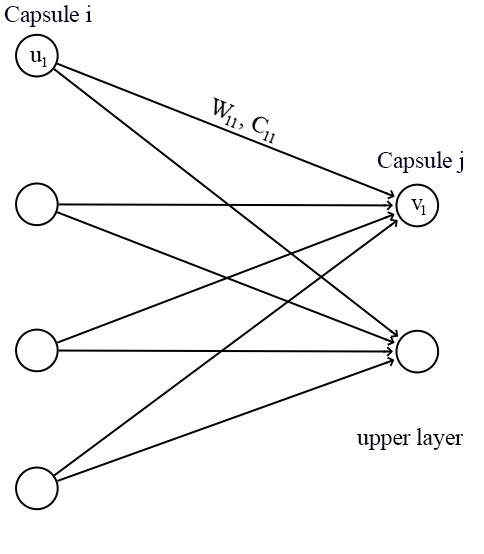
We apply a transformation matrix \(W_{ij}\) to the capsule output \(u_i\) of the pervious layer. For example, with a \(p \times k\) matrix, we transform \(u_i\) to \(\hat{u}_{j \vert i}\) from k-dimension to p-dimension. (\((p \times k) \times (k \times 1) \implies p \times 1\)) Then we compute a weighted sum \(s_j\) with weights \(c_{ij}\).
\[\begin{split} \hat{u}_{j|i} &= W_{ij} u_i \\ s_j & = \sum_i c_{ij} \hat{u}_{j|i} \\ \end{split}\]\(c_{ij}\) are coupling coefficients that are calculated by the iterative dynamic routing process (discussed next) and \(\sum_{j} c_{ij}\) are designed to sum to one. Conceptually, \(c_{ij}\) measures how likely capsule \(i\) may activate capsule \(j\).
Instead of applying a ReLU function, we apply a squashing function to \(s_j\) so the final output vector \(v_j\) of the capsule has length between 0 and 1. This function shrinks small vectors to zero and large vectors to unit vectors.
\[\begin{split} v_{j} & = \frac{\| s_{j} \|^2}{ 1 + \| s_{j} \|^2} \frac{s_{j}}{ \| s_{j} \|} \\ \end{split}\] \[\begin{split} v_{j} & \approx \| s_{j} \| s_{j} \quad & \text{for } s_{j} \text { is small. } \\ v_{j} & \approx \frac{s_{j}}{ \| s_{j} \|} \quad & \text{for } s_{j} \text { is large. } \\ \end{split}\]Iterative dynamic Routing
In capsule, we use iterative dynamic routing to compute the capsule output by calculating an intermediate value \(c_{ij}\) (coupling coefficient).
Recall that the prediction vector \(\hat{u}_{j \vert i}\) is computed as:
\[\begin{split} \hat{u}_{j|i} &= W_{ij} u_i \\ \end{split}\]and the activity vector \(v_j\) (the capsule \(j\) output) is:
\[\begin{split} s_j & = \sum_i c_{ij} \hat{u}_{j|i} \\ v_{j} & = \frac{\| s_{j} \|^2}{ 1 + \| s_{j} \|^2} \frac{s_{j}}{ \| s_{j} \|} \\ \end{split}\]Intuitively, prediction vector \(\hat{u}_{j \vert i}\) is the prediction (vote) from the capsule \(i\) on the output of the capsule \(j\) above. If the activity vector has close similarity with the prediction vector, we conclude that both capsules are highly related. Such similarity is measured using the scalar product of the prediction and the activity vector.
\[\begin{split} b_{ij} ← \hat{u}_{j \vert i} \cdot v_j \\ \end{split}\]Therefore, the similarity score \(b_{ij}\) takes into account on both likeliness and the feature properties, instead of just likeliness in neurons. Also, \(b_{ij}\) remains low if the activation \(u_i\) of capsule \(i\) is low since \(\hat{u}_{j \vert i}\) length is proportional to \(u_i\). i.e. \(b_{ij}\) should remain low between the mouth capsule and the face capsule if the mouth capsule is not activated.
The coupling coefficients \(c_{ij}\) is computed as the softmax of \(b_{ij}\):
\[\begin{split} c_{ij} & = \frac{\exp{b_{ij}}} {\sum_k \exp{b_{ik}} } \\ \end{split}\]To make \(b_{ij}\) more accurate , it is updated iteratively in multiple iterations (typically in 3 iterations).
\[\begin{split} b_{ij} ← b_{ij} + \hat{u}_{j \vert i} \cdot v_j \\ \end{split}\]Here is the final pseudo code for the dynamic routing:
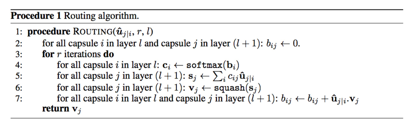
Source Sara Sabour, Nicholas Frosst, Geoffrey Hinton
Routing a capsule to the capsule in the layer above based on relevancy is called Routing-by-agreement.
The dynamic routing is not a complete replacement of the backpropagation. The transformation matrix \(W\) is still trained with the backpropagation using a cost function. However, we use dynamic routing to compute the output of a capsule. We compute \(c_{ij}\) to quantify the connection between a capsule and its parent capsules. This value is important but short lived. We re-initialize it to 0 for every datapoint before the dynamic routing calculation. To calculate a capsule output, training or testing, we always redo the dynamic routing calculation.
Max pooling shortcoming
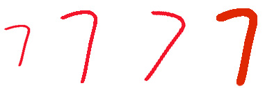
The max pooling in a CNN handles translational variance. Even a feature is slightly moved, if it is still within the pooling window, it can still be detected. Nevertheless, this approach keeps only the max feature (the most dominating) and throws away the others. Capsules maintain a weighted sum of features from the previous layer. Hence, it is more suitable in detecting overlapping features. For example detecting multiple overlapping digits in the handwriting:

Significant of routing-by-agreement with capsules
In a fully connected network, we calculate the neuron with
\[y_j = ReLU( \sum_{i} W_{ij} x_i + b_{j} ),\]and \(W\) is trained by the backpropagation with a global cost function. Iterative dynamic routing provides an alternative of calculating how a capsule is activated by using local features’ properties. Theoretically, we can group capsules better and simpler to form a parse tree with reduced risk of adversaries.
The iterative dynamic routing with capsules is just one showcase in demonstrating the routing-by-agreement. In a second paper on capsules Matrix capsules with EM routing, a matrix capsule [likeliness, 4x4 pose matrix] is proposed with a new Expectation-maximization (EM) routing. The pose matrices are designed to capture different viewpoints so a capsule can capture objects with different azimuths and elevations.
(Source from the paper Matrix capsules with EM routing)
Matrix capsules apply a clustering technique, the EM routing, to cluster related capsules to form a parent capsule. Even the viewpoint may change, the votes will change in a co-ordinate way from the red dots to the pink dots below. So the EM routing can still cluster the same children capsules together.
The first paper opens a new approach in the deep learning, and the second paper explores deeper into its potential. For those interested, there are more details in my second article on Matrix capsule.
CapsNet architecture
Finally, we apply capsules to build the CapsNet to classify the MNist digits. The following is the architecture using CapsNet.
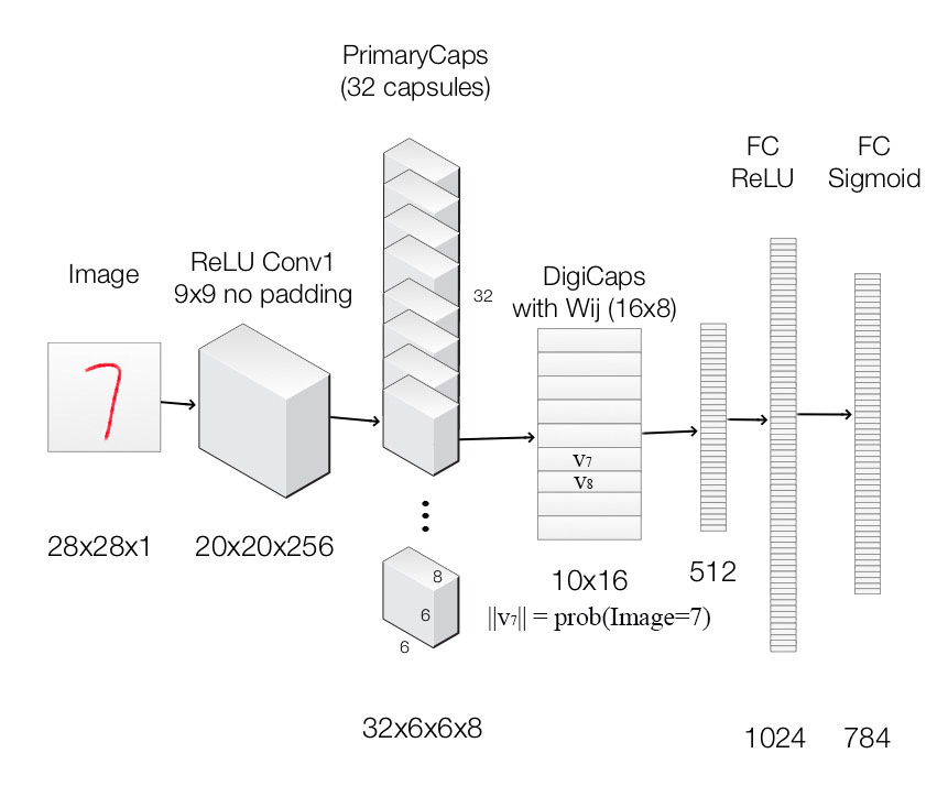
Image is feed into the ReLU Conv1 which is a standard convolution layer. It applies 256 9x9 kernels to generate an output with 256 channels (feature maps). With stride 1 and no padding, the spatial dimension is reduced to 20x20. ( 28-9+1=20)
It is then feed into PrimaryCapsules which is a modified convolution layer supporting capsules. It generates a 8-D vector instead of a scalar. PrimaryCapsules used 8x32 kernels to generate 32 8-D capsules. (i.e. 8 output neurons are grouped together to form a capsule) PrimaryCapsules uses 9x9 kernels with stride 2 and no padding to reduce the spatial dimension from 20x20 to 6x6 ( \(\lfloor \frac{20-9}{2} \rfloor + 1 = 6\)). In PrimaryCapsules, we have 32x6x6 capsules.
It is then feed into DigiCaps which apply a transformation matrix \(W_{ij}\) with shape 16x8 to convert the 8-D capsule to a 16-D capsule for each class \(j\) (from 1 to 10).
\[\begin{split} \hat{u}_{j|i} &= W_{ij} u_i \\ \end{split}\]The final output \(v_j\) for class \(j\) is computed as:
\[\begin{split} s_j & = \sum_i c_{ij} \hat{u}_{j|i} \\ v_{j} & = \frac{\| s_{j} \|^2}{ 1 + \| s_{j} \|^2} \frac{s_{j}}{ \| s_{j} \|} \\ \end{split}\]Because there are 10 classes, the shape of DigiCaps is 10x16 (10 16-D vector.) Each vector \(v_j\) acts as the capsule for class \(j\). The probability of the image to be classify as \(j\) is computed by \(\| v_j \|\). In our example, the true label is 7 and \(v_7\) is the latent representation of our input. With a 2 hidden fully connected layers, we can reconstruct the 28x28 image from \(v_7\).
Here is the summary of each layers:
| Layer Name | Apply | Output shape |
|---|---|---|
| Image | Raw image array | 28x28x1 |
| ReLU Conv1 | Convolution layer with 9x9 kernels output 256 channels, stride 1, no padding with ReLU | 20x20x256 |
| PrimaryCapsules | Convolution capsule layer with 9x9 kernel output 32x6x6 8-D capsule, stride 2, no padding | 6x6x32x8 |
| DigiCaps | Capsule output computed from a \(W_{ij}\) (16x8 matrix) between \(u_i\) and \(v_j\) (\(i\) from 1 to 32x6x6 and \(j\) from 1 to 10). | 10x16 |
| FC1 | Fully connected with ReLU | 512 |
| FC2 | Fully connected with ReLU | 1024 |
| Output image | Fully connected with sigmoid | 784 (28x28) |
Our capsule layers use convolution kernels to explore locality information.
Loss function (Margin loss)
In our example, we want to detect multiple digits in a picture. Capsules use a separate margin loss \(L_c\) for each category \(c\) digit present in the picture:
\[L_c = T_c \max(0, m^+ − \|v_c\|)^2 + λ (1 − T_c) \max(0, \|v_c\| − m^−)^2\]which \(T_c = 1\) if an object of class \(c\) is present. \(m^+ = 0.9\) and \(m^− = 0.1\). The λ down-weighting (default 0.5) stops the initial learning from shrinking the activity vectors of all classes. The total loss is just the sum of the losses of all classes.
Computing the margin loss in Keras
def margin_loss(y_true, y_pred):
    """
    :param y_true: [None, n_classes]
    :param y_pred: [None, num_capsule]
    :return: a scalar loss value.
    """
    L = y_true * K.square(K.maximum(0., 0.9 - y_pred)) + \
        0.5 * (1 - y_true) * K.square(K.maximum(0., y_pred - 0.1))

    return K.mean(K.sum(L, 1))
CapsNet model
Here is the Keras code in creating the CapsNet model:
def CapsNet(input_shape, n_class, num_routing):
    """
    :param input_shape: (None, width, height, channels)
    :param n_class: number of classes
    :param num_routing: number of routing iterations
    :return: A Keras Model with 2 inputs (image, label) and
             2 outputs (capsule output and reconstruct image)
    """
    # Image
    x = layers.Input(shape=input_shape)

    # ReLU Conv1
    conv1 = layers.Conv2D(filters=256, kernel_size=9, strides=1,
	             padding='valid', activation='relu', name='conv1')(x)

    # PrimaryCapsules: Conv2D layer with `squash` activation,
    # reshape to [None, num_capsule, dim_vector]
    primarycaps = PrimaryCap(conv1, dim_vector=8, n_channels=32,
	                    kernel_size=9, strides=2, padding='valid')

    # DigiCap: Capsule layer. Routing algorithm works here.
    digitcaps = DigiCaps(num_capsule=n_class, dim_vector=16,
	        num_routing=num_routing, name='digitcaps')(primarycaps)

    # The length of the capsule's output vector
    out_caps = Length(name='out_caps')(digitcaps)

    # Decoder network.
    y = layers.Input(shape=(n_class,))

    # The true label is used to extract the corresponding vj
    masked = Mask()([digitcaps, y])
    x_recon = layers.Dense(512, activation='relu')(masked)
    x_recon = layers.Dense(1024, activation='relu')(x_recon)
    x_recon = layers.Dense(784, activation='sigmoid')(x_recon)
    x_recon = layers.Reshape(target_shape=[28, 28, 1], name='out_recon')(x_recon)

    # two-input-two-output keras Model
    return models.Model([x, y], [out_caps, x_recon])
The length of the capsule’s output vector \(\| v_j \|\) corresponds to the probability that it belong to the class \(j\). For example, \(\| v_7 \|\) is the probability of the input image belongs to 7.
class Length(layers.Layer):
    def call(self, inputs, **kwargs):
        # L2 length which is the square root
        # of the sum of square of the capsule element
        return K.sqrt(K.sum(K.square(inputs), -1))
PrimaryCapsules
PrimaryCapsules converts 20x20 256 channels into 32x6x6 8-D capsules.
def PrimaryCap(inputs, dim_vector, n_channels, kernel_size, strides, padding):
    """
    Apply Conv2D `n_channels` times and concatenate all capsules
    :param inputs: 4D tensor, shape=[None, width, height, channels]
    :param dim_vector: the dim of the output vector of capsule
    :param n_channels: the number of types of capsules
    :return: output tensor, shape=[None, num_capsule, dim_vector]
    """
    output = layers.Conv2D(filters=dim_vector*n_channels, kernel_size=kernel_size, strides=strides, padding=padding)(inputs)
    outputs = layers.Reshape(target_shape=[-1, dim_vector])(output)
    return layers.Lambda(squash)(outputs)
Squash function
Squash function behaves like a sigmoid function to squash a vector such that its length falls between 0 and 1.
\[\begin{split} v_{j} & = \frac{\| s_{j} \|^2}{ 1 + \| s_{j} \|^2} \frac{s_{j}}{ \| s_{j} \|} \\ \end{split}\]def squash(vectors, axis=-1):
"""
The non-linear activation used in Capsule. It drives the length of a large vector to near 1 and small vector to 0
:param vectors: some vectors to be squashed, N-dim tensor
:param axis: the axis to squash
:return: a Tensor with same shape as input vectors
"""
s_squared_norm = K.sum(K.square(vectors), axis, keepdims=True)
scale = s_squared_norm / (1 + s_squared_norm) / K.sqrt(s_squared_norm)
return scale * vectors
DigiCaps with dynamic routing
DigiCaps converts the capsules in PrimaryCapsules to 10 capsules each making a prediction for class \(j\). The following is the code in creating 10 (n_class) 16-D (dim_vector) capsules:
# num_routing is default to 3
digitcaps = DigiCap(num_capsule=n_class, dim_vector=16,
                  num_routing=num_routing, name='digitcaps')(primarycaps)
DigiCap is just a simple extension of a dense layer. Instead of taking a scalar and output a scalar, it takes a vector and output a vector:
- input shape = (None, input_num_capsule (32), input_dim_vector(8) )
- output shape = (None, num_capsule (10), dim_vector(16) )
Here is the DigiCaps and we will detail some part of the code for explanation later.
class DigiCap(layers.Layer):
    """
    The capsule layer.

    :param num_capsule: number of capsules in this layer
    :param dim_vector: dimension of the output vectors of the capsules in this layer
    :param num_routings: number of iterations for the routing algorithm
    """
    def __init__(self, num_capsule, dim_vector, num_routing=3,
                 kernel_initializer='glorot_uniform',
                 b_initializer='zeros',
                 **kwargs):
        super(DigiCap, self).__init__(**kwargs)
        self.num_capsule = num_capsule    # 10
        self.dim_vector = dim_vector      # 16
        self.num_routing = num_routing    # 3
        self.kernel_initializer = initializers.get(kernel_initializer)
        self.b_initializer = initializers.get(b_initializer)

    def build(self, input_shape):
        "The input Tensor should have shape=[None, input_num_capsule, input_dim_vector]"
        assert len(input_shape) >= 3,
        self.input_num_capsule = input_shape[1]
        self.input_dim_vector = input_shape[2]

        # Transform matrix W
        self.W = self.add_weight(shape=[self.input_num_capsule, self.num_capsule,
                                 self.input_dim_vector, self.dim_vector],
                                 initializer=self.kernel_initializer,
                                 name='W')

        # Coupling coefficient.
        # The redundant dimensions are just to facilitate subsequent matrix calculation.
        self.b = self.add_weight(shape=[1, self.input_num_capsule, self.num_capsule, 1, 1],
                                    initializer=self.b_initializer,
                                    name='b',
                                    trainable=False)
        self.built = True

    def call(self, inputs, training=None):
        # inputs.shape = (None, input_num_capsule, input_dim_vector)
        # Expand dims to (None, input_num_capsule, 1, 1, input_dim_vector)
        inputs_expand = K.expand_dims(K.expand_dims(inputs, 2), 2)

        # Replicate num_capsule dimension to prepare being multiplied by W
        # Now shape = [None, input_num_capsule, num_capsule, 1, input_dim_vector]
        inputs_tiled = K.tile(inputs_expand, [1, 1, self.num_capsule, 1, 1])

        # Compute `inputs * W` by scanning inputs_tiled on dimension 0.
        # inputs_hat.shape = [None, input_num_capsule, num_capsule, 1, dim_vector]
        inputs_hat = tf.scan(lambda ac, x: K.batch_dot(x, self.W, [3, 2]),
                             elems=inputs_tiled,
                             initializer=K.zeros([self.input_num_capsule, self.num_capsule, 1, self.dim_vector]))
        # Routing algorithm
        assert self.num_routing > 0, 'The num_routing should be > 0.'
        for i in range(self.num_routing):
            c = tf.nn.softmax(self.b, dim=2)  # dim=2 is the num_capsule dimension
            # outputs.shape=[None, 1, num_capsule, 1, dim_vector]
            outputs = squash(K.sum(c * inputs_hat, 1, keepdims=True))

            # last iteration needs not compute b which will not be passed to the graph any more anyway.
            if i != self.num_routing - 1:
                self.b += K.sum(inputs_hat * outputs, -1, keepdims=True)
        return K.reshape(outputs, [-1, self.num_capsule, self.dim_vector])
build declares the self.W parameters representing the transform matrix W and self.b representing the \(b_{ij}\).
    def build(self, input_shape):
        "The input Tensor should have shape=[None, input_num_capsule, input_dim_vector]"
        assert len(input_shape) >= 3,
        self.input_num_capsule = input_shape[1]
        self.input_dim_vector = input_shape[2]

        # Transform matrix W
        self.W = self.add_weight(shape=[self.input_num_capsule, self.num_capsule,
                                 self.input_dim_vector, self.dim_vector],
                                 initializer=self.kernel_initializer,
                                 name='W')

        # Coupling coefficient.
        # The redundant dimensions are just to facilitate subsequent matrix calculation.
        self.b = self.add_weight(shape=[1, self.input_num_capsule, self.num_capsule, 1, 1],
                                    initializer=self.b_initializer,
                                    name='b',
                                    trainable=False)
        self.built = True
To compute:
\[\begin{split} \hat{u}_{j|i} &= W_{ij} u_i \\ \end{split}\]The code first expand the dimension of \(u_i\) and then multiple it with \(w\). Nevertheless, the simple dot product implementation of \(W_{ij} u_i\) (commet out below) is replaced by tf.scan for better speed performance.
class DigiCap(layers.Layer):
    ...

    def call(self, inputs, training=None):
        # inputs.shape = (None, input_num_capsule, input_dim_vector)
        # Expand dims to (None, input_num_capsule, 1, 1, input_dim_vector)
        inputs_expand = K.expand_dims(K.expand_dims(inputs, 2), 2)

        # Replicate num_capsule dimension to prepare being multiplied by W
        # Now shape = [None, input_num_capsule, num_capsule, 1, input_dim_vector]
        inputs_tiled = K.tile(inputs_expand, [1, 1, self.num_capsule, 1, 1])

        """
        # Compute `inputs * W`
        # By expanding the first dim of W.
        # W has shape (batch_size, input_num_capsule, num_capsule, input_dim_vector, dim_vector)
        w_tiled = K.tile(K.expand_dims(self.W, 0), [self.batch_size, 1, 1, 1, 1])

        # Transformed vectors,
        inputs_hat.shape = (None, input_num_capsule, num_capsule, 1, dim_vector)
        inputs_hat = K.batch_dot(inputs_tiled, w_tiled, [4, 3])
        """

        # However, we will implement the same code with a faster implementation using tf.sacn
        # Compute `inputs * W` by scanning inputs_tiled on dimension 0.
        # inputs_hat.shape = [None, input_num_capsule, num_capsule, 1, dim_vector]
        inputs_hat = tf.scan(lambda ac, x: K.batch_dot(x, self.W, [3, 2]),
                             elems=inputs_tiled,
                             initializer=K.zeros([self.input_num_capsule, self.num_capsule, 1, self.dim_vector]))
Here is the code to implement the following Iterative dynamic Routing pseudo code.
class DigiCap(layers.Layer):
    ...
    def call(self, inputs, training=None):
        ...
        # Routing algorithm
        assert self.num_routing > 0, 'The num_routing should be > 0.'

        for i in range(self.num_routing):  # Default: loop 3 times
            c = tf.nn.softmax(self.b, dim=2)  # dim=2 is the num_capsule dimension

            # outputs.shape=[None, 1, num_capsule, 1, dim_vector]
            outputs = squash(K.sum(c * inputs_hat, 1, keepdims=True))

            # last iteration needs not compute b which will not be passed to the graph any more anyway.
            if i != self.num_routing - 1:
                self.b += K.sum(inputs_hat * outputs, -1, keepdims=True)
        return K.reshape(outputs, [-1, self.num_capsule, self.dim_vector])
Image reconstruction
We use the true label to select \(v_j\) to reconstruct the image during training. Then we feed \(v_j\) through 3 fully connected layers to re-generate the original image.
Select \(v_j\) in training with Mask
class Mask(layers.Layer):
    """
    Mask a Tensor with shape=[None, d1, d2] by the max value in axis=1.
    Output shape: [None, d2]
    """
    def call(self, inputs, **kwargs):
        # use true label to select target capsule, shape=[batch_size, num_capsule]
        if type(inputs) is list:  # true label is provided with shape = [batch_size, n_classes], i.e. one-hot code.
            assert len(inputs) == 2
            inputs, mask = inputs
        else:  # if no true label, mask by the max length of vectors of capsules
            x = inputs
            # Enlarge the range of values in x to make max(new_x)=1 and others < 0
            x = (x - K.max(x, 1, True)) / K.epsilon() + 1
            mask = K.clip(x, 0, 1)  # the max value in x clipped to 1 and other to 0

        # masked inputs, shape = [batch_size, dim_vector]
        inputs_masked = K.batch_dot(inputs, mask, [1, 1])
        return inputs_masked
Reconstruction loss
A reconstruction loss \(\| \text{image} - \text{reconstructed image} \|\) is added to the loss function. It trains the network to capture the critical properties into the capsule. However, the reconstruction loss is multiple by a regularization factor (0.0005) so it does not dominate over the marginal loss.
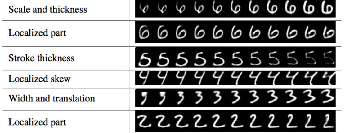
What capsule is learning?
Each capsule in DigiCaps is a 16-D vector. By slightly varying one dimension by holding other constant, we can learn what property for each dimension is capturing. Each row below is the reconstructed image (using the decoder) of changing only one dimension.
Sabour implementation
Sara Sabour released an implementation on Capsule at Github Sara Sabour. Since this is an ongoing research, do expect the implementation may be different from the paper.