“How to start a Deep Learning project?”
This is an archive for an article I posted on Medium on Deep Learning project. People interested in the article should read in my Medium blog since it has the latest updated version.
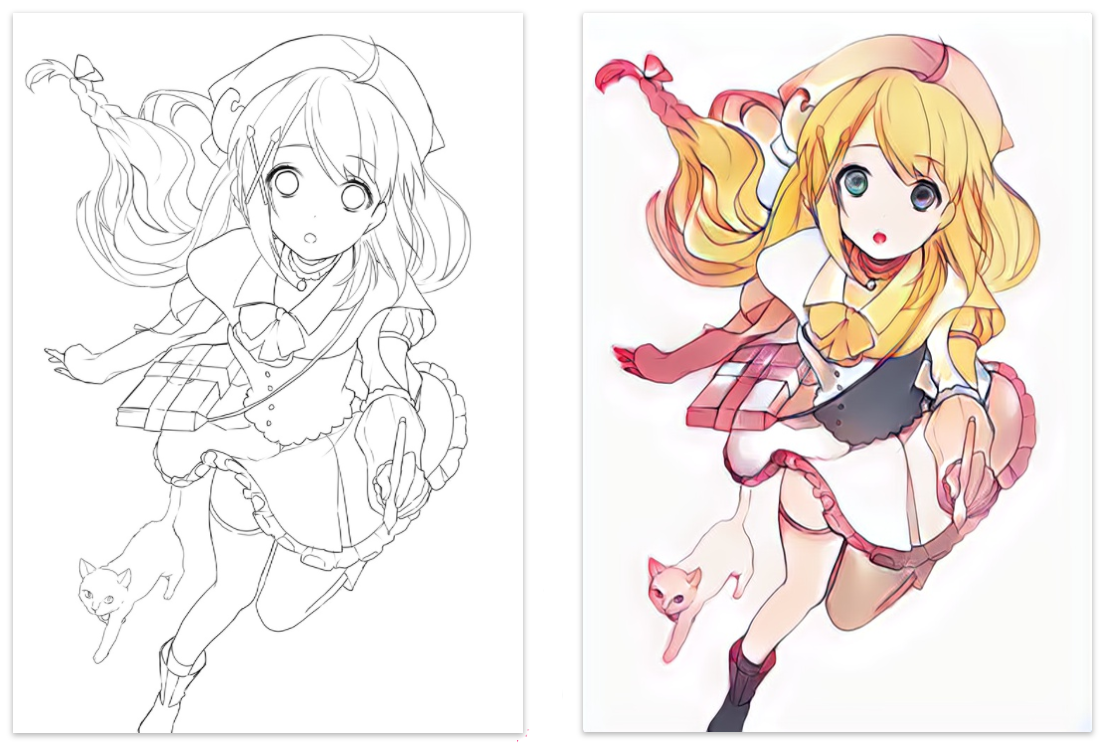
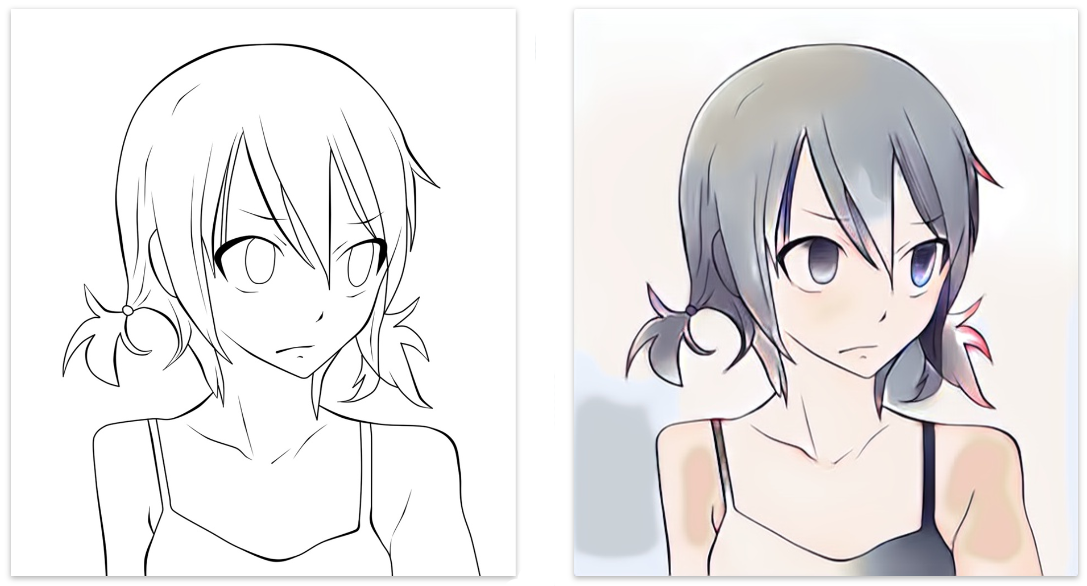
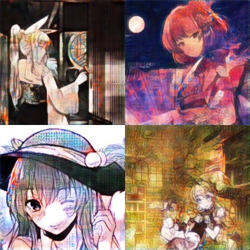
(Images generated from PaintsChainer.)
In this article, I will explain the whole journey from starting to finishing a deep learning (DL) project and illustrate the core ideas with a real project in colorizing line art. The whole series consists of six parts:
- Part 1: Start a Deep Learning project.
- Part 2: Build a Deep Learning dataset.
- Part 3: Deep Learning designs.
- Part 4: Visualize Deep Network models and metrics.
- Part 5: Debug a Deep Learning Network.
- Part 6: Improve Deep Learning Models performance & network tuning.
Part 1: Start a Deep Learning project
What projects to pick?
Many AI projects are not that serious and pretty fun. In early 2017, as part of my research on the topic of Generative Adversaries Network (GAN), I started a project to colorize Japanese Manga. The problem is difficult but it was fascinating in particular I cannot draw! In looking for projects, look beyond incremental improvements, make a product that is marketable, or create a new model that learns faster and better. Have fun and being innovative.
Debug Deep Network (DN) is tough
Deep Learning (DL) training composes of million iterations to build a model. Locate bugs are hard and it breaks easily. Start with something simple and make changes incrementally. Model optimizations like regularization can always wait after the code is debugged. Visualize your predictions and model metrics frequently. Make something works first so you have a baseline to fall back. Do not get stuck in a big model. It is more fun to see progress.
Start small, move small.
Measure and learn
Most personal projects last from two to four months for the first release. It is pretty short since research, debugging and experiments take time. We schedule those complex experiments to run overnight. By early morning, we want enough information to make our next move. As a good rule of thumb, those experiments should not run longer than 12 hours in the early phase. To achieve that, we narrow the scope to single Anime characters. As a flashback, we should reduce the scope further. We have many design tests and we need to turn around fast. Don’t plan too far ahead. We want to measure and learn fast.
Build, measure and learn.
Research v.s. product
When we start the Manga project in the Spring of 2017, Kevin Frans has a Deepcolor project to colorize Manga with spatial color hints using GAN.
Many AI fields are pretty competitive. When defining the goal, you want to push hard enough so the project is still relevant when it is done. GAN model is pretty complex and the quality is usually not product-ready in early 2017. Nevertheless, if you narrow what the product can handle smartly, you may push the quality high enough as a commercial product. To achieve that, select your training samples carefully. For any DL projects, strike a good balance among model generalization, capacity, and accuracy.
Cost
Training real-life models with a GPU is a must. It is 20 to 100 times faster than a CPU. The lowest price Amazon GPU p2.xlarge spot instance is about $7.5/day and then go up to $75/day for an 8 unit GPUs. Training models can be expensive consider that Google can spend a whole week in training NLP models using one thousand servers. In our Manga project, some experiments took over 2 days. We spend an average of $150/week. For faster iterations, it can ring up the bill to $1500/week with faster instances. Instead of using the cloud computing, you can purchase a standalone machine. A desktop with the Nvidia GeForce GTX 1080 TI costs about $2200 in Feb 2018. It is about 5x faster than a P2 instance in training a fine-tuned VGG model.
Time line
We define our development in four phases with the last 3 phases executed in multiple iterations.
- Project research
- Design
- Implementation and debugging
- Experiment and tuning
Project research
We do research in current offerings to explore their weakness. For many GAN type solutions, they utilized spatial color hints. The drawings are a little bit wash out or muddy. The colors sometimes bleed. We set a 2-month timeframe for our project with 2 top priorities: regenerate image without hints and improve color fidelity. Our goal is:
Color a grayscale Manga drawing without hints on single Anime characters.
Standing on the shoulders of giants
Then we study related research and open source projects. Spend a good amount of time in doing research. Gain intuitions on where existing models are flawed or performed well. Many people go through at least a few dozen papers and projects before starting their implementations. For example, when we deep down into GANs, there are over a dozen new GAN models: DRAGAN, cGAN, LSGAN etc… Reading research papers can be painful. Skim through the paper quickly to grab the core ideas. Pay attention to the figures. After knowing what is important, read the paper again.
Deep learning (DL) codes are condensed but difficult to troubleshoot. Research papers often miss details. Many projects start off with implementations that show successes for similar problems. Search hard. Try a few options. We locate code implementations on different GAN variants. We trace the code and give them a few test drives. We replace the generative network of one implementation with an image encoder and a decoder. As a special bonus, we find the hyperparameters in place are pretty decent. Otherwise, searching for the initial hyperparameters can be tedious when the code is still buggy.
Part 2: Build a Deep Learning dataset
Dataset
Garbage in and garbage out. Good data trains good models.
Public and academic datasets
For research projects, search for established public datasets. Those datasets have cleaner samples and published model performance that you can baseline on. If you have more than one options, select the one with the highest quality samples relevant to your problems.
Custom datasets
For real-life problems, we need samples originated from the problem domains. Try to locate public datasets first. The efforts to build a high-quality custom dataset is rarely discussed properly. If none is available, search where you can crawl the data. Usually, there are plenty suggestions, but the data quality is usually low. Evaluate all your options for quality before crawling samples.
A high-quality dataset should contain:
- balanced taxonomy.
- sufficient amount of data.
- minimum data and label’s noise.
- relevant to your problems.
- diversify.
Do not crawl all your data at once. Train and test run samples in your model and refine the crawled taxonomy from lessons learned. The crawled dataset also requires significant cleanup. Otherwise, even with the best model designs, it will still fall short of human-level performance. Danbooru and Safebooru are two very popular sources of Anime characters. But some deep learning applications prefer Getchu for better quality drawings. We can download drawings from Safebooru using a set of tags. We examine the samples visually and run tests to analyze the errors (the samples that perform badly). Both the model training and the manual evaluation provide further information to refine our tag selections. With continue iterations, we learn more and build our samples gradually. Download files to different folders according to the tags or categories such that we can merge them later based on our experience. We need to clean up samples. Some projects use a classifier to further filter samples not relevant to the problem. For example, remove all drawings with multiple characters. Some projects use Illustration2Vec to estimate tags by extracting features from the drawings and use this information for fine-tuned filtering. Smaller projects rarely collect as many samples comparing with academic datasets. Apply transfer learning if needed.
I re-visit the progress on the Manga colorization when I write this article. Deepcolor was inspired by PaintsChainer. We did not spend much time on PaintsChainer when we started the project. But I am glad to play them a visit.
The left drawing is provided by PaintsChainer and the right is the drawing colored by the machine. Definitely, this is product-ready quality.
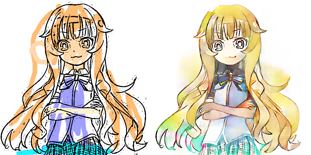
We decided to test it with some of our training samples. It is less impressive. Fewer colors are applied and the style is not correct.
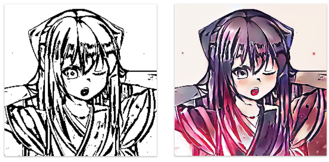
Since we trained our model for a while, we knew what drawings will perform badly. As expected, it has a hard time for drawings with entangled structures.
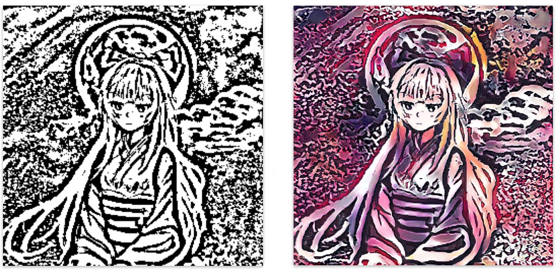
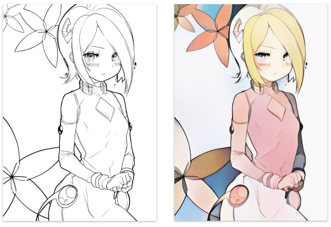
This illustrates a very important point: choose your samples well. As a product offering, PaintsChainer makes a smart move on focusing the type of scratches that they excel. To proof that I use a clean line art picked from the internet. The result is impressive again.
There are a few lessons learned here. There is no bad data, just the data is not solving your needs. Focus on what your product wants to offer. As samples’ taxonomy increased, it is much harder to train and to maintain output quality.
In early development, we realize some drawings have too many entangled structures. Without significantly increasing the model capacity, those drawings produce little values in training and better be left off. It just makes the training inefficient.
Trim out irrelevant data. You will get a better model.
To recap,
- Use public dataset if possible.
- Find the best site(s) for high quality and diversify samples.
- Categorize samples into folders and merge your data based on the lessons learned.
- Analyze errors and filter out samples irrelevant to your real-life problem.
- Build your samples iteratively.
- Balanced the number of samples for each class.
- Shuffle your samples before training.
- Collect sufficient samples. If not, apply transfer training.
Part 3: Deep Learning designs
Simple and smart
Start your design simple and small. In the study phase, people are flooded with many cool ideas. We tend to code all the bots and nuts in one shoot. This will not work. Try to beat the state-of-the-art too early is not practical. Ironically, trying to beat the odds of random guessing first. Design with fewer layers and customizations. Delay solutions that require un-necessary hyperparameters tuning. Verify the loss is dropping and check whether the model shows signs of “intelligence”. Do not waste time training the model with too many iterations or too large batch size. After a short debugging, our model produces pretty un-impressive results after 5000 iterations. But colors start confined to regions. There is hope that skin tone is showing up.

This gives us valuable feedback on whether the model starts coloring. Do not start with something big. You will spend most of your time debugging this or wondering do we just need another hour to train the model.
Nevertheless, this is easier to say than doing it. We jump steps. But you are warned!
Priority & incremental driven design
To create simple designs first, we need to sort out the top priorities. We should break down complex problems into smaller problems and solve them in steps. Our first design involves convolutions, transposed convolutions, and a discriminative network. This may be too complex as a first design. But since we only redesigned the discriminative network from a tested GAN implementation, it is still manageable. To maximize the chance of success, we analyze what is our top issue. GAN is hard to train. From our previous experience, we know the gradient diminishing problem will be an issue for us. So we research a couple skip connections to mitigate the problem.
Everyone has a plan ‘till they get punched in the mouth. (a quote form Mike Tyson) The right strategy in a DL project is to maneuver quickly from what you see. Before jumping to a model using no hints, we start with one with spatial color hints. We do not move to a “no hint” design in one step. We first move to a model with color hints but dropping the hints’ spatial information. The color quality drops significantly. We know our priority is shifted. We refine our deep learning (DN) model first before making the next big jump. Instead of making a long-term plan that keeps changing, adopt a shorter lean process driven by priorities. Model changes usually have many surprises, bugs and new issues. Use shorter and smaller design iterations to make it manageable.
Transfer learning with pre-trained models
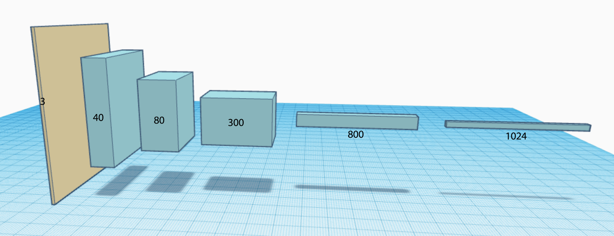
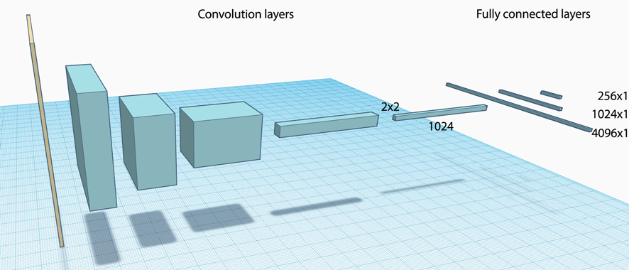
Training from scratch takes a long time. As stated from the VGG paper in 2014: the VGG model was originally trained with four NVIDIA Titan Black GPUs, training a single net took 2–3 weeks depending on the architecture. Training a complex CNN model like VGG19 with a small dataset will overfit the model. Alternatively, we can design a smaller model to improve generalization. For some problems, it is not feasible. We need a complex model to extract complex latent factors. To overcome the overfitting problem, we fine-tune pre-trained model (like VGG19 or ResNet) using our sample data. This can repurpose the network in shorter time and fewer data. Usually, the first few convolution layers perform common tasks like edges and color detection. We can freeze those layers from updates. We can further speed up the training at the cost of accuracy if we retrain the last few fully connected layers only. Because we start with pretty good model parameters, we often use smaller learning rate also. Pre-trained models can be used across multiple disciplines. Indeed, we can model the Chinese language with a pre-trained English model.
Constraints
From the Boltzmann machine to the Restricted Boltzmann machine, we apply constraints to the network design to make training more effective. Building deep learning is not only putting layers together. Adding good constraints make learning more efficient or more “intelligent”. In our design, we apply denoising to restrict the amount of information that the spatial color hints may provide. We purposely soften those hints or corrupt it by zeroing a large fraction of hints. Ironically, it generalizes the model better and less sensitive to variants.
DL is more than adding layers.
Design details
For the rest of the article, we discuss some of the most common design decisions encounter in a DL project.
Cost function and metrics
Not all cost functions are created equally. It impacts how easy to train the model. Some cost functions are pretty standard, but some problem domains need some careful thoughts.
| Problems | Cost functions |
|---|---|
| Classification | Cross entropy, SVM |
| Regression | Mean square error (MSE) |
| Object detection or segmentation | Intersection over Union (IoU) |
| Policy optimization | Kullback–Leibler divergence |
| Word embedding | Noise Contrastive Estimation (NCE) |
| Word vectors | Cosine similarity |
Cost functions looking good in the theoretical analysis may not perform well in practice. For example, the cost function for the discriminator network in GAN adopts a more practical and empirical approach than the theoretical one. In some problem domains, the cost functions can be part guessing and part experimental. It can be a combination of a few cost functions. In our project, we start with the standard GAN cost functions. We also add a reconstruction cost using MSE and other regularization costs. However, our brain does not judge styling by MSE. One of the unresolved areas in our project is to find a better reconstruction cost function. We believe it will have a significant impact on the color fidelity.
Finding good cost functions becomes more important when we move into less familiar problem domains.
Good metrics help you to compare and tune models better. Search for established metrics for your type of problem. Unfortunately, for our project, it is very hard to define a precise accuracy formula for artistic rendering.
Regularization
L1 and L2 regularization are both common but L2 regularization is more popular in DL.
L1 regularization promotes sparsity in parameters. Sparsity encourages representations that disentangle the underlying representation. Since each non-zero parameter adds a penalty to the cost, it prefers more zero parameters than the L2 regularization. i.e. it prefers many zeros and a slightly larger parameter than many tiny parameters in L2 regularization. L1 regularization makes filters cleaner and therefore easier to interpret. L1 regularization is good for the feature selection. Since sparse models can be optimized easier and therefore consume less power, L1 is more suitable for the mobile device. L1 is also less vulnerable to outliners and works better if the data is less clean. However, L2 regularization remains more popular because the solution may be more stable.
Dropout can be applied to the fully connected layers as another regularization technique in large networks. The benefit of combining dropout with L2 regularization, if any, is domain specific. Usually, we apply those techniques in fine-tuning and we collect empirical data to verify its benefit. Generally, we start tuning the dropout rate from 20% and gradually increase it up to 50% until the model is just slightly overfitted.
Gradient descent
Always monitor gradient closely for diminishing or exploding gradients. Gradient descent problems have many possible causes which are very hard to verify. Do not jump into the learning rate tuning or making model design changes too fast. In early debugging, the small gradients may simply cause by programming bugs. For example, the input data is not scaled properly, or the weights are all initialized to zero. Tuning takes time. It will have better returns if we have verified other causes first.
If other possible causes are eliminated, apply gradient clipping (in particular for NLP) when gradient explode. Skip connections are a common technique to mitigate gradient diminishing problem. In ResNet, a residual layer allows the input to bypass the current layer to the next layer. Effectively, it reduces the depth of the network to make training easier in early training.
Scaling
We often scale input features using a mean and a variance computed from the training dataset. When we scale the validation or testing data, do not recompute them. We reuse the same mean and the variance from the training dataset. If features are not scaled correctly, we will either have exploding or diminishing gradients.
Batch Normalization & Layer Normalization
Apply batch normalization (BN) to CNN. DN learns faster and better if inputs are properly normalized. In BN, we compute the means and the variances for each location from each batch of training data. For example, with a batch size of 16 and a feature map with 10x10 spatial dimension, we compute 100 means and 100 variances (one per location). The mean at each location is the average of the corresponding locations from the 16 samples. We use the means and the variances to renormalize the node outputs at each location. BN improves accuracy and reduces training time. As a side bonus, we can increase the learning rate further to make training faster.
However, BN is not effective for RNN. We use Layer normalization instead. In RNN, the means and variances from the BN are not suitable to renormalize the output of RNN cells. It is likely because of the recurrent nature of the RNN and the sharing parameters. In Layer normalization, the output is renormalized by the mean and the variance calculated by the layer’s output of the current sample. A 100 elements layer uses only one mean and one variance from the current input to renormalize the layer.
Activation functions
In DL, ReLU is the most popular activation function to introduce non-linearity to the model. If the learning rate is too high, many nodes can be dead and stay dead. If changing the learning rate does not help, we can try leaky ReLU or PReLU. In a leaky ReLU, instead of outputting zero when x < 0, it has a small predefined downward slope (say 0.01 or set by a hyperparameter). Parameter ReLU (PReLU) pushes a step further. Each node will have a trainable slope.
Split dataset
To test the real performance, we split our data into three parts: 70% for training, 20% for validation and 10% for testing. Make sure samples are randomized properly in each dataset and each batch of training samples. During training, we use the training dataset to build models with different hyperparameters. We run those models with the validation dataset and pick the one with the highest accuracy. This strategy works if the validation dataset is similar to what we want to predict. But, as the last safeguard, we use the 10% testing data for a final insanity check. This testing data is for a final verification, but not for model selection. If your testing result is dramatically different from the validation result, the data should be randomized more, or more data should be collected.
Baseline
Setting a baseline helps us in comparing models and debugging. Research projects often require an established model as a baseline to compare models. For example, we can have a VGG19 model as the baseline for classification problems. Alternatively, we can extend some established and simple models to solve our problem first. This helps us to understand the problem better and establishes a performance baseline for comparison. This baseline implementation can also be used to validate data processing codes. In our project, we modify an established GAN implementation and redesign the generative network as our baseline.
Checkpoints
We save models’ output and metrics periodically for comparison. Sometimes, we want to reproduce results for a model or reload a model to train it further. Checkpoints allow us to save models to be reloaded later. However, if the model design has changed, all old checkpoints cannot be loaded. Even there is no automated process to solve this, we use Git tagging to trace multiple models and reload the correct model for a specific checkpoint. Checkpoints in TensorFlow is huge. our designs take 4 GB per checkpoint. When working in a cloud environment, configure enough storages accordingly. We start and terminate Amazon cloud instances frequently. Hence, we store all the files in the Amazon EBS so it can be reattached easily.
DL framework
In just six months after the release of TensorFlow from Google on Nov 2015, it became the most popular deep learning framework. While it seems implausible for any challengers soon, PyTorch was released by Facebook a year later and get a lot of traction from the research community. As of 2018, there are many choices of deep learning platform including TensorFlow, PyTorch, Caffe, Caffe2, MXNet, CNTK etc… In TensorFlow, you build a computation graph and submit it to a session later for computation. In PyTorch, every computation is executed immediately. TensorFlow’s approach creates a black box that makes debugging in-convenient. That is why tf.print becomes so dominant in debugging TensorFlow. The TensorFlow approach should be easier to optimize but yet we have not seen the speed up as it may indicate. Nevertheless, the competition is so fierce that any feature comparison will be obsolete in months. For example, Google already released an alpha version of eager execution in v1.5 to address this issue. But there is one key factor triggers the defection of some researchers to PyTorch. The PyTorch design is end-user focused. The API is simple and intuitive. The error messages make sense and the documentation is well organized. The pre-trained model and data pre-processing in PyTorch are very popular. TensorFlow does a great job in matching features. But so far, it adopts a bottom-up approach that makes things un-necessary complex. It may provide better flexibility but many of them are rarely used. The design thinking in TensorFlow can be chaotic. For example, it has about half a dozen API model to build DN: the result of many consolidations and matching competitor offerings.
Make no mistakes, TensorFlow is still dominating as of Feb 2018. The developer community is still much bigger. This may be the only factor matters. If you want to train the model with hundred machines or deploy the inference engine onto a mobile phone, TensorFlow is the only choice. Nevertheless, if other platforms prove themselves to provide what end-user needs, we will foresee more deflection for small to mid-size projects. For researchers preferring a simple API, TensorFlow also provides a Keras API to build DN.
Custom layers
Built-in layers from DL software packages are better tested and optimized. Nevertheless, if custom layers are needed:
- Unit test the forward pass and backpropagation code with non-random data.
- Compare the backpropagation result with the naive gradient check.
- Add tiny ϵ for the division or log computation to avoid NaN.
Randomization
One of the challenges in DL is reproducibility. During debugging, if the initial model parameters keep changing between sessions, it will be hard to debug. Hence, we explicitly initialize the seeds for all randomizer. In our project, we initialize the seeds for python, the NumPy and the TensorFlow. For final tuning, we turn off the explicit seed initialization so we generate different models for each run. To reproduce the result of a model, we checkpoint a model and reload it later.
Optimizer
Adam optimizer is one of the most popular optimizers in DL, if not the most popular. It suits many problems including models with sparse or noisy gradients. It achieves good results fast with the greatest benefit of easy tuning. Indeed, default configuration parameters often do well. Adam optimizer combines the advantages of AdaGrad and RMSProp. Instead of one single learning rate for all parameters, Adam internally maintains a learning rate for each parameter and separately adapt them as learning unfolds. Adam is momentum based using a running record of the gradients. Therefore, the gradient descent runs smoother and it dampens the parameter oscillation problem due to the large gradient and learning rate. A less popular option is the SGD using Nesterov Momentum.
Adam optimizer tuning
Adam has 4 configurable parameters.
- The learning rate (default 0.001)
- β1 is the exponential decay rate for the first moment estimates (default 0.9).
- β2 is the exponential decay rate for the second-moment estimates (default 0.999). This value should be set close to 1.0 on problems with a sparse gradient.
- ϵ(default 1e-8) is a small value added to the mathematical operation to avoid illegal operations like divide by zero.
β (momentum) smoothes out the gradient descent by accumulate information on the previous descent to smooth out the gradient changes. The default configuration works well for early development usually. If not, the most likely parameter to be tuned is the learning rate.
Part 4: Visualize Deep Network models and metrics
Never shot in the dark. Make an educated guess.
We fall into the hype of Deep Learning (DL). We exaggerate how easy DL is by counting the lines of code. This is deceptive. During troubleshooting, we see people jumping into leads without supporting evidence and wasting hours of efforts. It is important to track every move and to examine results at each step. With the help of pre-built package like TensorFlow, visualize the model and metrics is easy and the rewards are almost instantaneously.
Data visualization (input, output)
Verifying the input and the output of the model. Before feeding data into a model, save some training and validation samples for visual verification. Apply steps to undo the data pre-processing. Rescale the pixel value back to [0, 255]. Check a few batches to verify we are not repeating the same batch of data. The left side images below are some training samples and the right is a validation sample.

Sometimes, it is nice to verify the input data’s histogram. Ideally, it should be zero-centered ranging from -1 to 1.
(Source Sung Kim)
Save the corresponding model’s outputs regularly for verification and error analysis.

Metrics (Loss & accuracy)
Besides logging the loss and the accuracy to the stdout regularly, we record and plot them to analyze its long-term trend. The diagram below is the accuracy and the cross entropy loss displayed by the TensorBoard.
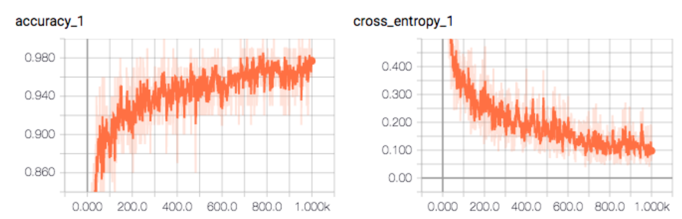
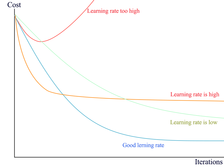
Plotting the cost helps us to tune the learning rate. Any prolonged jump in cost indicates the learning rate is too high. If it is too low, we learn slowly.
Here is another real example when the learning rate is too high. We see a sudden surge in loss (likely caused by a sudden jump in the gradient).
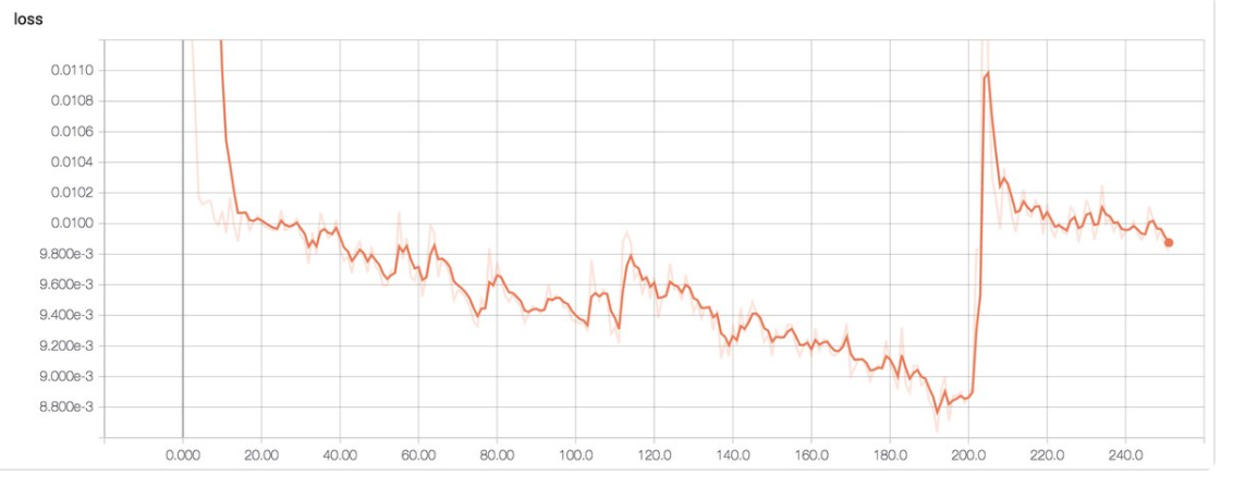
(Image source Emil Wallner)
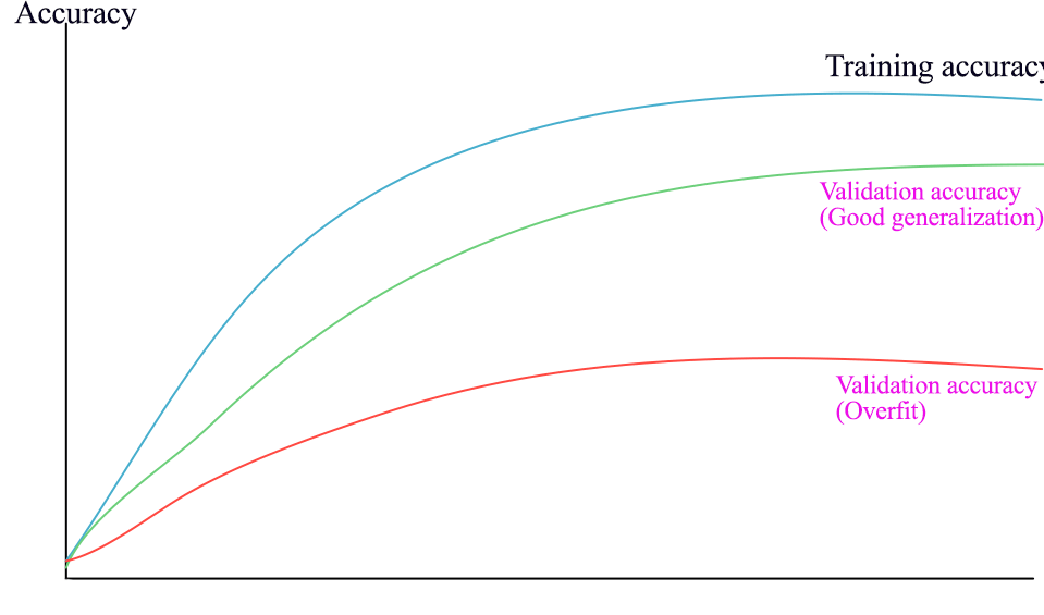
We use the plot on accuracy to tune regularization factors. If there is a major gap between the validation and the training accuracy, the model is overfitted. To reduce overfitting, we increase regularizations.
History summary
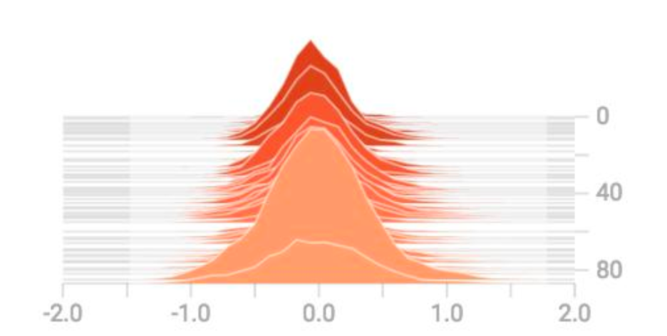
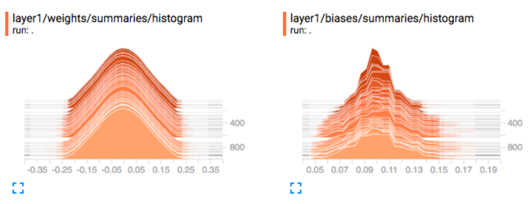
Weight & bias: We monitor the weights and the biases closely. Here are the Layer 1’s weights and biases distributions at different training iterations. Finding large (positive or negative) weights or bias is abnormal. A Normal distributed weight is a good sign that the training is going well (but not absolutely necessary).
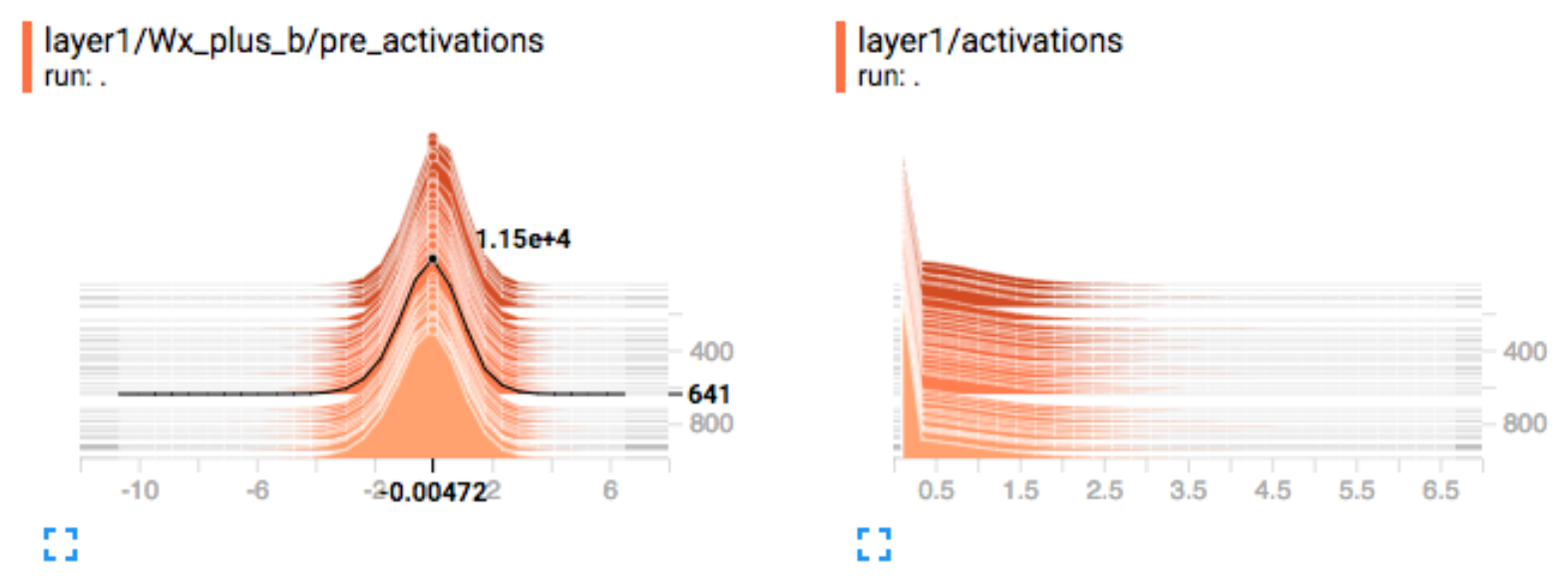
Activation: For gradient descent to perform the best, the nodes’ outputs before the activation functions should be Normal distributed. If not, we should apply a batch normalization to convolution layers or a layer normalization to RNN layers. We also monitor the number of dead nodes (zero activations) after the activation functions.
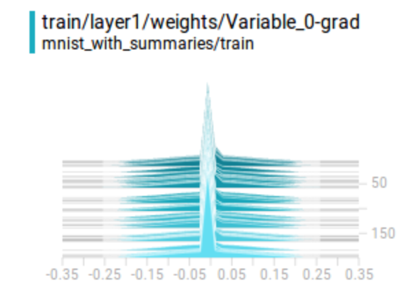
Gradients: For each layer, we monitor the gradients to identify one of the most serious DL problems: gradient diminishing or exploding problems. If gradients diminish quickly from the rightmost layers to the leftmost layers, we have a gradient diminishing problem.
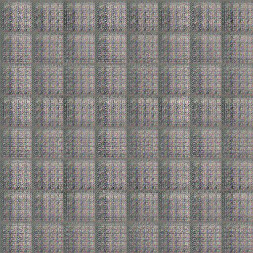
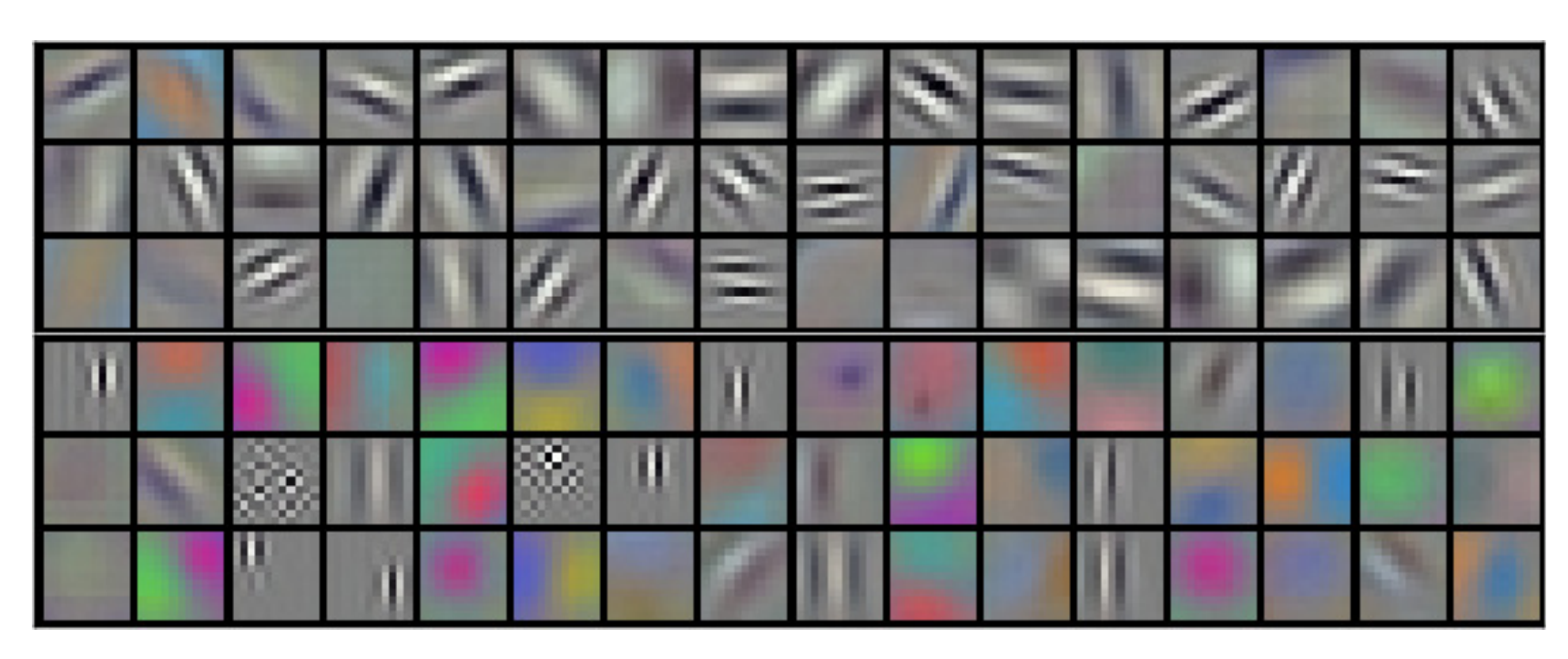
Not very common, we visualize the CNN filters. It identifies the type of features that the model is extracting. As shown below, the first couple convolution layers are detecting edges and colors.
For CNN, we can visualize what a feature map is learning. In the following picture, it captures the top 9 pictures (on the right side) having the highest activation in a particular map. It also applies a deconvolution network to reconstruct the spatial image (left picture) from the feature map.
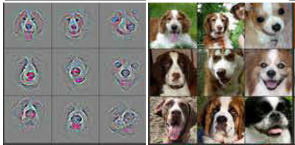
(Source: Visualizing and Understanding Convolutional Networks, Matthew D Zeiler et al.)
This image reconstruction is rarely done. But in a generative model, we often vary just one latent factor while holding others constant, It verifies whether the model is learning anything smart.
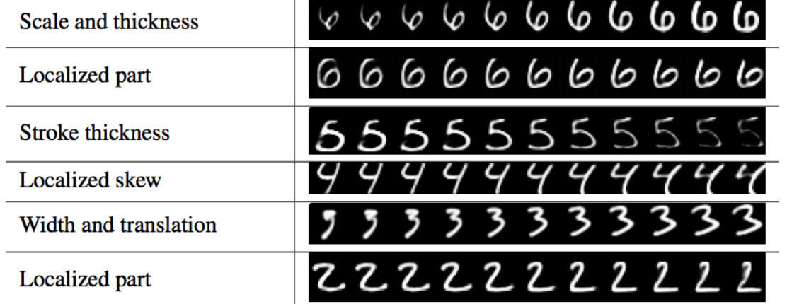
(Source Dynamic Routing Between Capsules, Sara Sabour, Nicholas Frosst, Geoffrey E Hinton)
Part 5: Debug a Deep Learning Network
In the early development, we are fighting multiple battles at the same time. As mentioned before, Deep Learning (DL) training composes of million iterations to build a model. Locate bugs are hard and it breaks easily. Start with something simple and make changes incrementally. Model optimizations like regularization can always wait after the code is debugged. Implement only the core part of the model with minimum customizations. Focus on verifying the model is functioning first.
- Set the regularization factors to zero.
- No other regularization (including dropouts).
- Use the Adam optimizer with default settings.
- Use ReLU.
- No data augmentation.
- Fewer DN layers.
- Scale your input data but no un-necessary pre-processing.
- Don’t waste time in long training iterations or large batch size.
Overfitting the model with a small amount of training data is the best way to debug. If the loss does not drop within a few thousand iterations, debug the code further. Achieve your first milestone by beating the odds of guessing. Then make incremental modifications to the model: add more layers and customization. Train it with the full training dataset. Add regularizations to control the overfit by monitor the accuracy gap between the training and validation dataset.
If stuck, take out all bells and whistles and make your problem smaller.
Initial hyperparameters
Many hyperparameters are more relevant to the model optimization. Turn them off or use default values. Use Adam optimizer. It is fast, efficient and the default learning rate does well. Early problems are mostly from bugs rather from the model design or tuning problems. Go through the checklist in the next section before any tunings. It is more common and easier to verify. If loss still does not drop after verifying the checklist, tune the learning rate. If the loss drops too slow, increase the learning rate by 10. If the loss goes up or the gradient explodes, decrease the learning rate by 10. Repeat the process until the loss drops gradually and nicely. Typical learning rates are between 1 and 1e-7.
Checklist
Data:
- Visualize and verify the input data (after data pre-processing and before feeding to the model).
- Verify the accuracy of the input labels (after data shuffle if applicable).
- Do not feed the same batch of data over and over.
- Scale your input properly (likely between -1 and 1 and zero centered).
- Verify the range of your output (e.g. between -1 and 1).
- Always use the mean/variance from the training dataset to rescale the validation/testing dataset.
- All input data to the model has the same dimensions.
- Access the overall quality of the dataset. (Are there too many outliners or bad samples?)
Model:
- The model parameters are initialized correctly. The weights are not set to all 0.
- Debug layers that the activations or gradients diminish/explode. (from rightmost to leftmost layers)
- Debug layers that weights are mostly zero or too large.
- Verify and test your loss function.
- For pre-trained model, your input data range matches the range used in the model.
- Dropout in inference and testing should be always off.
Weight initialization
Initialize the weights to all zeros is one of the most common mistakes and the DN will never learn anything. Weights should be initialized with a Gaussian distribution:

Scaling & normalization
Improper scaling is another major source of problems. If input features and nodes output follow a Normal distribution, the model will be much easier to train. If it is not done correctly, the loss will not drop regardless of the learning rate. We should monitor the histogram for the input features and the nodes’ outputs for each layer (before the activation functions). Always scale input properly. If the nodes’ outputs are not zero-centered and the model has training problems, apply batch normalization for CNN and layer normalization for RNN.
Loss function
Verify and test the correctness of your loss function. The loss of your model must be lower than the one from the random guessing. For example, in a classification problem with 10 classes, the cross entropy loss for random guessing is -ln(1/10).
Analysis errors
Review what is doing badly (errors) and improve it. Visualize your errors. In our project, the model performs badly for images with highly entangled structure. Identify the model weakness to make changes. For example, add more convolution layers with smaller filters to disentangle small features. Augment data if necessary, or collect more similar samples to train the model better. In some situations, you may want to remove those samples and constrain yourself to a more focus model.
Regularization tuning
Turn off regularization (overfit the model) until it makes reasonable predictions.
Once the model code is working, the next tuning parameters are the regularization factors. We increase the volume of our training data and then increase the regularizations to narrow the gap between the training and the validation accuracy. Do not overdo it as we want a slightly overfit model to work with. Monitor both data and regularization cost closely. Regularization loss should not dominate the data loss over prolonged periods. If the gap does not narrow with very large regularizations, debug the regularization code or method first.
Similar to the learning rate, we change testing values in the logarithmic scale. (for example, change by a factor of 10 at the beginning) Beware that each regularization factor can be in a totally different order of magnitude, and we may tune those parameters back and forth.
Multiple cost functions
For the first implementations, avoid using multiple data cost functions. The weight for each cost function may be in different order of magnitude and will require some efforts to tune it. If we have only one cost function, it can be absorbed into the learning rate.
Frozen variables
When we use pre-trained models, we may freeze those model parameters in certain layers to speed up computation. Double check no variables are frozen in-correctly.
Unit testing
As less often talked, we should unit test core modules so the implementation is less vulnerable to code changes. Verify the output of a layer may not be easy if its parameters are initialized with a randomizer. Otherwise, we can mock the input data and verify the outputs. For each module (layers), We can verify
- the shape of the output in both training and inference.
- the number of trainable variables (not the number of parameters).
Dimension mismatch
Always keep track of the shape of the Tensor (matrix) and document it inside the code. For a Tensor with shape [N, channel, W, H ], if W (width) and H (height) are swapped, the code will not generate any error if both have the same dimension. Therefore, we should unit test our code with a non-symmetrical shape. For example, we unit test the code with a [4, 3] Tensor instead of a [4, 4] Tensor.
Part 6: Improve Deep Learning Models performance & network tuning
Once we have our models debugged, we can focus on the model capacity and the hyperparameters tuning.
Increase model capacity
To increase the capacity, we add layers and nodes to a DN gradually. Deeper models produce more complex models. We also reduce filter sizes for convolution layers. Smaller filters (3x3 or 5x5) usually perform better than larger filters.
The tuning process is more empirical than theoretical. We add layers and nodes gradually with the intention to overfit the model since we can tone it down with regularizations. We repeat the iterations until the validation accuracy improvement is diminishing and no longer justify the drop in the training and computation performance.
However, GPUs do not page out memory. As of early 2018, the high-end NVIDIA GeForce GTX 1080 TI has 11GB memory. The maximum number of hidden nodes between two affine layers is restricted by the memory size.
For very deep networks, the gradient diminishing problem is serious. We add skip connection design (like the residual connections in ResNet) to mitigate the problem.
Model & dataset design changes
Here is the checklist to improve performance:
- Analyze errors (bad predictions) in the validation dataset.
- Monitor the activation. Consider batch or layer normalization if it is not zero centered.
- Monitor the percentage of dead nodes.
- Apply gradient clipping (in particular NLP) to control exploding gradients.
- Shuffle dataset (manually or programmatically).
- Balance the dataset (Each class has the similar amount of samples).
If the DN has a huge amount of dead nodes, we should trace the problem further. It can be caused by bugs, weight initializations or diminishing gradients. If none is true, experiment some advance ReLU functions like leaky ReLU.
Dataset collection & cleanup
One of the most effective ways to avoid overfitting and to improve performance is collecting more training data. We should analyze the errors. In our project, images with highly entangled structure perform badly. We can change the model by adding convolution layers with smaller filters. We can also collect more entangled samples for further training. Alternatively, we can limit what the model can handle. Remove those samples (outliners) so the training can be more focus. Custom dataset requires much more resources to build.
Data augmentation
Collect labeled data is expensive. For images, we can apply data augmentation with simple techniques like rotation, clipping, shifting, shear and flipping to create more samples from existing data. For example, if low contrast images are not performing, we can augment existing images to include different levels of contrast.

We can also supplement training data with non-labeled data. We use our model to classify data. For samples with high confidence prediction, we add them to the training dataset with the corresponding label predictions.
Tuning
Learning rate tuning
Let’s have a short recap on tuning the learning rate. In early development, we turn off or set to zero for any non-critical hyperparameters including regularizations. With the Adam optimizer, the default learning rate usually works well. If we are confident in the code but yet the loss does not drop, start tuning the learning rate. The typical learning rate is from 1 to 1e-7. Drop the rate each time by a factor of 10. Test it in short iterations. Monitor the loss closely. If it goes up consistently, the learning rate is too high. If it does not go down, the learning rate is too low. Increase it until the loss prematurely flattens.
The following is a real example showing the learning rate is too high and cause a sudden surge in cost with the Adam optimizer:
(source Emil Wallner)
In a less often used practice, people monitor the updates to W ratio:

- If the ratio is > 1e-3, consider lowering the learning rate.
- If the ratio is < 1e-3, consider increasing the learning rate.
Hyperparameters tuning
Once the model design is stabled, we can tune the model further. The most tuned hyperparameters are:
- Mini-batch size
- Learning rate
- Regularization factors
- Layer-specific hyperparameters (like dropout)
Mini-batch size
Typical batch size is either 8, 16, 32 or 64. If the batch size is too small, the gradient descent will not be smooth. The model is slow to learn and the loss may oscillate. If the batch size is too high, the time to complete one training iteration (one round of update) will be long with relatively small returns. For our project, we drop the batch size lower because each training iteration takes too long. We monitor the overall learning speed and the loss closely. If it oscillates too much, we know we are going too far. Batch size impacts hyperparameters like regularization factors. Once we determine the batch size, we usually lock the value.
Learning rate & regularization factors
We can tune our learning rate and regularization factors further with the approach mentioned before. We monitor the loss to control the learning rate and the gap between the validation and the training accuracy to adjust the regularization factors. Instead of changing the value by a factor of 10, we change that by a factor of 3 (or even smaller in the fine tuning).
Tuning is not a linear process. Hyperparameters are related, and we will come back and forth in tuning hyperparameters. Learning rate and regularization factors are highly related and may need to tune them together sometimes. Do not waste time in fine tuning too early. Design changes easily void such efforts.
Dropout
The dropout rate is typically from 20% to 50%. We can start with 20%. If the model is overfitted, we increase the value.
Other tuning
- Sparsity
- Activation functions
Sparsity in model parameters make computation optimization easier and it reduces power consumption in particular for mobile devices. If needed, we may replace the L2 regularization with the L1 regularization. ReLU is the most popular activation function. For some deep learning competitions, people experiment more advanced variants of ReLU to move the bar slightly higher. It also reduces dead nodes in some scenarios.
Advance tuning
There are more advanced fine tunings.
- Learning rate decay schedule
- Momentum
- Early stopping
Instead of a fixed learning rate, we can decay the learning rate regularly. The hyperparameters include how often and how much it drops. For example, you can have a 0.95 decay rate for every 100,000 iterations. To tune these parameters, we monitor the cost to verify it is dropping faster but not pre-maturely flatten.
Advance optimizers use momentum to smooth out the gradient descent. In the Adam optimizer, there are two momentum settings controlling the first order (default 0.9) and the second order (default 0.999) momentum. For problem domains with steep gradients like NLP, we may increase the value slightly.
Overfitting can be reduced by stopping the training when the validation errors increase persistently.
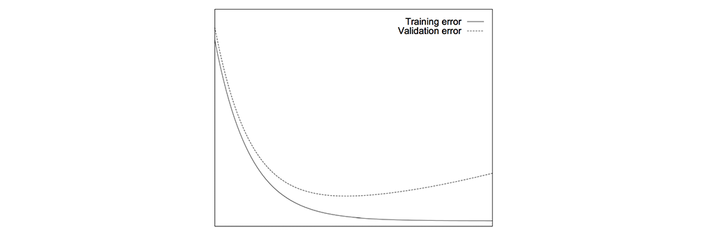
However, this is just a visualization of the concept. The real-time error may go up temporarily and then drop again. We can checkpoint models regularly and log the corresponding validation errors. Later we select the model.
Grid search for hyperparameters
Some hyperparameters are strongly related. We should tune them together with a mesh of possible combinations on a logarithmic scale. For example, for 2 hyperparameters λ and γ, we start from the corresponding initial value and drop it by a factor of 10 in each step:
- (e-1, e-2, … and e-8) and,
- (e-3, e-4, … and e-6).
The corresponding mesh will be [(e-1, e-3), (e-1, e-4), … , (e-8, e-5) and (e-8, e-6)].
Instead of using the exact cross points, we randomly shift those points slightly. This randomness may lead us to some surprises that otherwise hidden. If the optimal point lays in the border of the mesh (the blue dot), we retest it further in the border region.

A grid search is computationally intense. For smaller projects, this is used sporadically. We start tuning parameters in coarse grain with fewer iterations. To fine-tune the result, we use longer iterations and drop values by a factor of 3 (or even smaller).
Model ensembles
In machine learning, we can take votes from a number of decision trees to make predictions. It works because mistakes are often localized: there is a smaller chance for two models making the same mistakes. In DL, we start training with random guesses (providing random seeds are not explicitly set) and the optimized models are not unique. We pick the best models after many runs using the validation dataset. We take votes from those models to make final predictions. This method requires running multiple sessions and can be prohibitively expensive. Alternatively, we run the training once and checkpoints multiple models. We pick the best models from the checkpoints. With ensemble models, the predictions can base on:
- one vote per model,
- weighted votes based on the confidence level of its prediction.
Model ensembles are very effective in pushing the accuracy up a few percentage points in some problems and very common in some DL competitions.
Model improvement
Instead of fine-tuning a model, we can try out different model variants to leapfrog the model performance. For example, we have considered replacing the color generator partially or completely with an LSTM based design. This concept is not completely foreign: we draw pictures in steps.
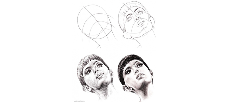
Intuitively, there are merits in introducing a time sequence method in image generation. This method has proven some success in DRAW: A Recurrent Neural Network For Image Generation.
Fine tune vs model improvement
Major breakthroughs require model design changes. However, some studies indicate fine-tuning a model can be more beneficial than making incremental model changes. The final verdicts are likely based on your own benchmarking results.
Kaggle
You may have a simple question like should I use Leak ReLU. It sounds so simple but you will never get a straight answer anywhere. Some research papers show empirical data that leaky ReLU is superior, but yet some projects see no improvement. There are too many variables and many projects do not have the resources to benchmark even a portion of the possibilities. Kaggle is an online platform for data science competitions including deep learning. Dig through some of the competitions and you can find the most common performance metrics. Some teams also publish their code (called kernels). With some patience, it is a great source of information.
Experiment framework
DL requires many experiments and tuning hyperparameters is tedious. Creating an experiment framework can expedite the process. For example, some people develop code to externalize the model definitions into a string for easy modification. Those efforts are usually counterproductive for a small team. I personally find the drop in code simplicity and traceability is far worse than the benefit. Such coding makes simple modification harder than it should be. Easy to read code has fewer bugs and more flexible. Instead, many AI cloud offerings start providing automatic hyperparameters tuning. It is still in an infant state but it should be the general trend that we do not code the framework ourselves. Stay tuned for any development!