“TensorFlow Basic - tutorial.”
Basic
TensorFlow is an open source software platform for deep learning developed by Google. This tutorial is designed to teach the basic concepts and how to use it. This article is intended for audiences with some simple understanding on deep learning.
First TensorFlow program
TensorFlow represents computations by linking op (operation) nodes into a computation graph. TensorFlow programs are structured into a construction phase and an execution phase. The following program:
- Constructs a computation graph for a matrix multiplication.
- Open a TensorFlow session and execute the computation graph.
import tensorflow as tf

# Construct 2 ops representing 2 matrices.
# All ops are automatically added to the default computation graph.
# tf.constant outputs a Tensor and assign it to m1 or m2.
m1 = tf.constant([[3, 5]])     # shape: (1, 2)
m2 = tf.constant([[2],[4]])    # shape: (2, 1)

# Create a matrix multiplication op
# Assign the output Tensor to "product".
product = tf.matmul(m1, m2)

with tf.Session() as sess:     # Open a session to execute the default graph.
    result = sess.run(product) # Compute the result for “product”
    print(result)              # 3*2+5*4: [[26]]
sess.run(product) returns a NumPy array containing the result of the computation.
Tensor & Computation graph
TensorFlow builds a computation graph containing ops (operation nodes). It usually starts with an op that takes in a list or a placeholder with data provided later.
m1 = tf.constant([[3, 5]])
tf.constant builds an op that represents a Python list. By default, all ops are added to the current default graph.
Ops output zero or more Tensors. In TensorFlow, a Tensor is a typed multi-dimensional array, similar to a Python list or a NumPy ndarray. The shape of a tensor is its dimension. For example, a 5x5x3 matrix is a Rank 3 (3-dimensional) tensor with shape (5, 5, 3). Because our list is a 1x2 array of type int32, it outputs a Tensor of type int32 with shape (2, ): a 1-dimensional array with 2 elements.
We make additional TensorFlow calls to link ops and tensors together to form a graph. tf.matmul links 2 tensors to create a matrix multiplication tensor.
product = tf.matmul(m1, m2)    # A matrix multiplication operation takes 2 Tensors
                               # and output 1 Tensor
During these calls, no actual computations are done. All computations are delayed until we invoke a Tensor inside a session (sess.run). Then all the required operations to compute the Tensor will be executed.
with tf.Session() as sess:     # Open a session to execute the default graph.
    result = sess.run(product) # Compute the result for “product”
With TensorFlow v1.5, the eager execution model executes ops immediately. It is not released for production yet. We will discuss this model later.
Common ops to hold data are:
- tf.Variable
- tf.Constant
- tf.Placeholder
- tf.SparseTensor
tf.placeholder
tf.constant hardwires the input matrices as constant ops. These constants are part of the computation graph running with the same input. To switch to different input data, we replace the constant ops with the placeholders. When we run a graph in a session, we feed different input matrices into the placeholders using feed_dict.
x = tf.placeholder(tf.int32, shape=(2, 1))
b = tf.placeholder(tf.int32)
...
with tf.Session() as sess:
    result = sess.run(product, feed_dict={x: np.array([[2],[4]]), b:1})
    ...
Here is the full source code:
import tensorflow as tf
import numpy as np

W = tf.constant([[3, 5]])

# Allow data to be supplied later during execution.
x = tf.placeholder(tf.int32, shape=(2, 1))
b = tf.placeholder(tf.int32)

# A linear model y = Wx + b
product = tf.matmul(W, x) + b

with tf.Session() as sess:
    # Feed data into the place holder (x & b) before execution.
    result = sess.run(product, feed_dict={x: np.array([[2],[4]]), b:1})
    print(result)              # 3*2+5*4+1 = [[27]]

    result = sess.run(product, feed_dict={x: np.array([[5],[6]]), b:3})
    print(result)              # [[48]]
By default, the data type (dtype) of a tensor is tf.float32. In our code, we explicitly define the type to be int32 in tf.placeholder.
Train a linear model
Let’s build a simple linear regression model: with training data \(x\) and labels \(y\). We want to build a linear model and find (train) the parameters \(W\) and \(b\).
\[y = Wx + b\]The code implementation contains 3 major parts:
- Define a model
- Define a loss function and an optimizer for the gradient descent
- Train the model
Model
Define the linear model y = Wx + b.
### Define a model: a computational graph
# Parameters for a linear model y = Wx + b
W = tf.get_variable("W", initializer=tf.constant([0.1]))
b = tf.get_variable("b", initializer=tf.constant([0.0]))

# Placeholder for input and prediction
x = tf.placeholder(tf.float32)
y = tf.placeholder(tf.float32)

# Define a linear model y = Wx + b
model = W * x + b
We define both \(W\) and \(b\) as TensorFlow variables initialized to 0.1 and 0.0 respectively. By default, TensorFlow variables are trainable and used to define models’ parameters.
W = tf.get_variable("W", initializer=tf.constant([0.1]))
b = tf.get_variable("b", initializer=tf.constant([0.0]))
Variables produce Tensor outputs. Tensors can be multi-dimensional. The code below creates a variable with shape (5, 5, 3) of type int32, and we use a zero initializer to set all values to 0.
int_v = tf.get_variable("my_int_variable_name", [5, 5, 3], dtype=tf.int32,
  initializer=tf.zeros_initializer)
Lost function and optimizer & trainer
To define the Mean Square Error (MSE) cost function, we subtract the label value from the prediction of a model, and then sum over its square.
loss = tf.reduce_sum(tf.square(model - y))
We create a gradient descent optimizer and a trainer to find the optimal trainable parameters \(W\) and \(b\) for our model.
# Optimizer with a 0.01 learning rate
optimizer = tf.train.GradientDescentOptimizer(0.01)
train = optimizer.minimize(loss)
Training
All operations are not yet executed. Before any execution, we need to initialize all the variables first.
tf.global_variables_initializer().run()
It actually runs all the initialization ops of all variables inside a session. This is a short cut for:
init = tf.global_variables_initializer()
with tf.Session() as sess:
    sess.run(init)
We train our model with 1000 iterations. For every 100 iterations, we compute the loss and print it out.
for i in range(1000):
   sess.run(train, {x:x_train, y:y_train})
   if i%100==0:
        l_cost = sess.run(loss, {x:x_train, y:y_train})
        print(f"i: {i} cost: {l_cost}")
After 1000 iterations are done, we stop the training, and print out W, b and the loss:
# Evaluate training accuracy
l_W, l_b, l_cost  = sess.run([W, b, loss], {x:x_train, y:y_train})
print(f"W: {l_W} b: {l_b} cost: {l_cost}")

# W: [ 1.99999797] b: [-0.49999401] cost: 2.2751578399038408e-11
From the printout, we realize the model trained from our data is:
\[y = 2x - 0.5\]Here is the full source code:
import tensorflow as tf

### Define a model: a computational graph
# Parameters for a linear model y = Wx + b
W = tf.get_variable("W", initializer=tf.constant([0.1]))
b = tf.get_variable("b", initializer=tf.constant([0.0]))

# Placeholder for input and prediction
x = tf.placeholder(tf.float32)
y = tf.placeholder(tf.float32)

# Define a linear model y = Wx + b
model = W * x + b

### Define a cost function, an optimizer and a trainer
# Define a cost function (Mean square error - MSE)
loss = tf.reduce_sum(tf.square(model - y))

# Optimizer with a 0.01 learning rate
optimizer = tf.train.GradientDescentOptimizer(0.01)
train = optimizer.minimize(loss)

### Training (Fitting)
# Training data
x_train = [1.0, 2.0, 3.0, 4.0]
y_train = [1.5, 3.5, 5.5, 7.5]

with tf.Session() as sess:
    # Retrieve the variable initializer op and initialize variable W & b.
    sess.run(tf.global_variables_initializer())
    for i in range(1000):
        sess.run(train, {x:x_train, y:y_train})
        if i%100==0:
            l_cost = sess.run(loss, {x:x_train, y:y_train})
            print(f"i: {i} cost: {l_cost}")

    # Evaluate training accuracy
    l_W, l_b, l_cost  = sess.run([W, b, loss], {x:x_train, y:y_train})
    print(f"W: {l_W} b: {l_b} cost: {l_cost}")
    # W: [ 1.99999797] b: [-0.49999401] cost: 2.2751578399038408e-11
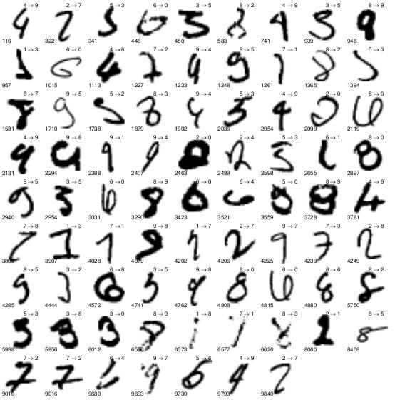
Solving MNist
The MNIST dataset contains handwritten digits with examples shown as above. It has a training set of 60,000 examples and a test set of 10,000 examples. The following python file from TensorFlow mnist_softmax.py train a linear classifier for MNist digit recognition. The following model reaches an accuracy of 92%.
import argparse
import sys

from tensorflow.examples.tutorials.mnist import input_data

import tensorflow as tf

FLAGS = None


def main(_):
  # Import data
  mnist = input_data.read_data_sets(FLAGS.data_dir)

  # Create the model
  x = tf.placeholder(tf.float32, [None, 784])

  W = tf.get_variable("W", [784, 10], initializer=tf.zeros_initializer)
  b = tf.get_variable("b", [10], initializer=tf.zeros_initializer)

  y = tf.matmul(x, W) + b

  # Define loss and optimizer
  y_ = tf.placeholder(tf.int64, [None])

  cross_entropy = tf.losses.sparse_softmax_cross_entropy(labels=y_, logits=y)
  train_step = tf.train.GradientDescentOptimizer(0.5).minimize(cross_entropy)

  sess = tf.InteractiveSession()
  tf.global_variables_initializer().run()

  # Train
  for _ in range(1000):
    batch_xs, batch_ys = mnist.train.next_batch(100)
    sess.run(train_step, feed_dict={x: batch_xs, y_: batch_ys})

  # Test trained model
  correct_prediction = tf.equal(tf.argmax(y, 1), y_)
  accuracy = tf.reduce_mean(tf.cast(correct_prediction, tf.float32))
  print(sess.run(
      accuracy, feed_dict={
          x: mnist.test.images,
          y_: mnist.test.labels
      }))


if __name__ == '__main__':
  parser = argparse.ArgumentParser()
  parser.add_argument(
      '--data_dir',
      type=str,
      default='/tmp/tensorflow/mnist/input_data',
      help='Directory for storing input data')
  FLAGS, unparsed = parser.parse_known_args()
  tf.app.run(main=main, argv=[sys.argv[0]] + unparsed)

# 0.9198
We use an already made library to read training, validation and testing dataset into “mnist”.
from tensorflow.examples.tutorials.mnist import input_data

mnist = input_data.read_data_sets(FLAGS.data_dir)
Each image is 28x28 = 784. We use a linear classifier to classify the handwritten image to one of the 10 classes. (with output 0 to 9)
x = tf.placeholder(tf.float32, [None, 784])
W = tf.get_variable("W", [784, 10], initializer=tf.zeros_initializer)
b = tf.get_variable("b", [10], initializer=tf.zeros_initializer)
y = tf.matmul(x, W) + b
We use cross-entropy as the cost functions:
cross_entropy = tf.losses.sparse_softmax_cross_entropy(labels=y_, logits=y)
Solving MNist with a fully connected networking
Now we replace the model using deep learning techniques. This example contains 2 hidden fully connected layers. The new model achieves an accuracy of 97%.
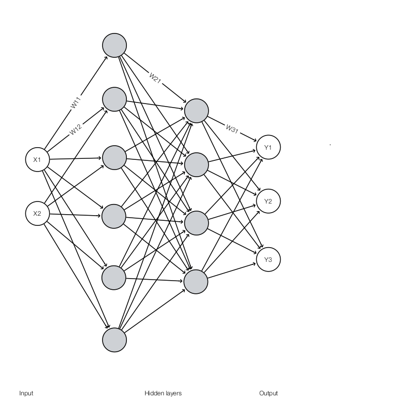
To implement a fully connected layer:
\[\begin{split} z & = Wx + b\\ h & = ReLU(z) \\ \end{split}\]We creates 2 trainable variables \(W\) and \(b\). We compute \(Wx + b\) and then apply the ReLU function:
with tf.variable_scope('hidden1'):
  weights = tf.get_variable("W", [784, 128],
  				initializer=tf.truncated_normal_initializer(stddev=0.1))
  biases = tf.get_variable("b", [128], initializer=tf.zeros_initializer)
  z = tf.matmul(x, weights) + biases
  hidden1 = tf.nn.relu(z)
In our model, we have 2 fully connected hidden layers and one linear output layer. We also apply the He initialization for stddev.
def mnist_fc(x):
  # First fully connected net
  with tf.variable_scope('hidden1'):
    weights = tf.get_variable("W", [784, 128],
          initializer=tf.truncated_normal_initializer(stddev=np.sqrt(2.0 / 784)))
    biases = tf.get_variable("b", [128], initializer=tf.zeros_initializer)
    hidden1 = tf.nn.relu(tf.matmul(x, weights) + biases)

  # Second fully connected net
  with tf.variable_scope('hidden2'):
    weights = tf.get_variable("W", [128, 32],
          initializer=tf.truncated_normal_initializer(stddev=np.sqrt(2.0 / 128)))
    biases = tf.get_variable("b", [32], initializer=tf.zeros_initializer)
    hidden2 = tf.nn.relu(tf.matmul(hidden1, weights) + biases)

  # Linear
  with tf.variable_scope('softmax_linear'):
    weights = tf.get_variable("W", [32, 10],
          initializer=tf.truncated_normal_initializer(stddev=np.sqrt(2.0 / 32)))
    biases = tf.get_variable("b", [10], initializer=tf.zeros_initializer)
    logits = tf.nn.relu(tf.matmul(hidden2, weights) + biases)

  return logits
We use cross entropy for our cost function and Adam optimizer as our trainer:
# Model

x = tf.placeholder(tf.float32, [None, 784])
y_labels = tf.placeholder(tf.int64, [None])

y = mnist_fc(x)

# Loss, optimizer and trainer

with tf.name_scope('loss'):
  cross_entropy = tf.losses.sparse_softmax_cross_entropy(
      labels=y_labels, logits=y)
cross_entropy = tf.reduce_mean(cross_entropy)

with tf.name_scope('adam_optimizer'):
  train_step = tf.train.AdamOptimizer(1e-4).minimize(cross_entropy)
For every 100 iterations, we also evaluate the accuracy of the model by computing the mean of correct predictions. (for example, 0.93)
# Evaluation
with tf.name_scope('accuracy'):
  correct_prediction = tf.equal(tf.argmax(y, 1), y_labels)
  correct_prediction = tf.cast(correct_prediction, tf.float32)
accuracy = tf.reduce_mean(correct_prediction)
Here is the full source code:
import argparse
import sys
import numpy as np

from tensorflow.examples.tutorials.mnist import input_data

import tensorflow as tf

FLAGS = None


def mnist_fc(x):
  # First fully connected net
  with tf.variable_scope('hidden1'):
    weights = tf.get_variable("W", [784, 128],
          initializer=tf.truncated_normal_initializer(stddev=np.sqrt(2.0 / 784)))
    biases = tf.get_variable("b", [128], initializer=tf.zeros_initializer)

    hidden1 = tf.nn.relu(tf.matmul(x, weights) + biases)

  # Second fully connected net
  with tf.variable_scope('hidden2'):
    weights = tf.get_variable("W", [128, 32],
          initializer=tf.truncated_normal_initializer(stddev=np.sqrt(2.0 / 128)))
    biases = tf.get_variable("b", [32], initializer=tf.zeros_initializer)

    hidden2 = tf.nn.relu(tf.matmul(hidden1, weights) + biases)

  # Linear
  with tf.variable_scope('softmax_linear'):
    weights = tf.get_variable("W", [32, 10],
          initializer=tf.truncated_normal_initializer(stddev=np.sqrt(2.0 / 32)))
    biases = tf.get_variable("b", [10], initializer=tf.zeros_initializer)

    logits = tf.nn.relu(tf.matmul(hidden2, weights) + biases)

  return logits


def main(_):
  # Import data
  mnist = input_data.read_data_sets(FLAGS.data_dir)

  # Model

  x = tf.placeholder(tf.float32, [None, 784])
  y_labels = tf.placeholder(tf.int64, [None])

  y = mnist_fc(x)

  # Loss, optimizer and trainer

  with tf.name_scope('loss'):
    cross_entropy = tf.losses.sparse_softmax_cross_entropy(
        labels=y_labels, logits=y)
  cross_entropy = tf.reduce_mean(cross_entropy)

  with tf.name_scope('adam_optimizer'):
    train_step = tf.train.AdamOptimizer(1e-4).minimize(cross_entropy)

  # Evaluation
  with tf.name_scope('accuracy'):
    correct_prediction = tf.equal(tf.argmax(y, 1), y_labels)
    correct_prediction = tf.cast(correct_prediction, tf.float32)
  accuracy = tf.reduce_mean(correct_prediction)

  with tf.Session():
    tf.global_variables_initializer().run()
    for i in range(20000):
      batch = mnist.train.next_batch(50)
      train_step.run(feed_dict={x: batch[0], y_labels: batch[1]})

      if i % 100 == 0:
        train_accuracy = accuracy.eval(feed_dict={x: batch[0], y_labels: batch[1]})
        print('step %d, training accuracy %g' % (i, train_accuracy))

    print('test accuracy %g' % accuracy.eval(feed_dict={
        x: mnist.test.images, y_labels: mnist.test.labels}))

if __name__ == '__main__':
  parser = argparse.ArgumentParser()
  parser.add_argument('--data_dir', type=str,
                      default='/tmp/tensorflow/mnist/input_data',
                      help='Directory for storing input data')
  FLAGS, unparsed = parser.parse_known_args()
  tf.app.run(main=main, argv=[sys.argv[0]] + unparsed)
Further accuracy improvement can be achieved by:
- Increase the number of training iterations.
- Change to a CNN model.
- Add L2 regularization into the cost function.
- Add batch normalization or dropout.
- Fine tuning the learning rate and the \(\lambda\) in the L2 regularization.
In next section, we will cover the CNN and dropout implementation.
MNist with a Convolution network (CNN)
To push the accuracy higher, we create a model with :
- 1st CNN layer using 5x5 filter with strides 1 and 32 output channels
- 2nd CNN layer (32 channels -> 64 channels)
- One hidden fully connected layer of (7x7x65 -> 1024)
- Output fully connected layer (1024 -> 10 classes)
- Use cross entropy cost function with Adam optimizer.
It reaches an accuracy of 99.4% with little parameter tuning.
Each convolution layer includes:
- tf.nn.conv2d to perform the 2D convolution
- tf.nn.relu for the ReLU
- tf.nn.max_pool for the max pool.
with tf.variable_scope('conv1'):
  W_conv1 = tf.get_variable("W", [5, 5, 1, 32],
        initializer=tf.truncated_normal_initializer(stddev=np.sqrt(2.0 / 784)))
  b_conv1 = tf.get_variable("b", initializer=tf.constant(0.1, shape=[32]))
  z = tf.nn.conv2d(x_image, W_conv1, strides=[1, 1, 1, 1], padding='SAME')
  z += b_conv1
  h_conv1 = tf.nn.relu(z + b_conv1)

# Pooling layer - downsamples by 2X.
with tf.variable_scope('pool1'):
  h_pool1 = tf.nn.max_pool(h_conv1, ksize=[1, 2, 2, 1],
                   strides=[1, 2, 2, 1], padding='SAME')
We also apply tf.nn.dropout (Dropout) to regulate the first hidden layer:
# Dropout - regulate the complexity of the model
with tf.variable_scope('dropout'):
  keep_prob = tf.placeholder(tf.float32)
  h_fc1_drop = tf.nn.dropout(h_fc1, keep_prob)
Here is the full source code:
import argparse
import sys
import tempfile
import numpy as np

from tensorflow.examples.tutorials.mnist import input_data

import tensorflow as tf

FLAGS = None


def deepnn(x):
  with tf.name_scope('reshape'):
    x_image = tf.reshape(x, [-1, 28, 28, 1])

  # First convolutional layer - maps one grayscale image to 32 feature maps.
  with tf.variable_scope('conv1'):
    W_conv1 = tf.get_variable("W", [5, 5, 1, 32],
          initializer=tf.truncated_normal_initializer(stddev=np.sqrt(2.0 / 784)))
    b_conv1 = tf.get_variable("b", initializer=tf.constant(0.1, shape=[32]))
    z = tf.nn.conv2d(x_image, W_conv1, strides=[1, 1, 1, 1], padding='SAME')
    z += b_conv1
    h_conv1 = tf.nn.relu(z + b_conv1)

  # Pooling layer - downsamples by 2X.
  with tf.variable_scope('pool1'):
    h_pool1 = tf.nn.max_pool(h_conv1, ksize=[1, 2, 2, 1],
                     strides=[1, 2, 2, 1], padding='SAME')

  # Second convolutional layer -- maps 32 feature maps to 64.
  with tf.variable_scope('conv2'):
    W_conv2 = tf.get_variable("W", [5, 5, 32, 64],
          initializer=tf.truncated_normal_initializer(stddev=np.sqrt(2.0 / 32)))
    b_conv2 = tf.get_variable("b", initializer=tf.constant(0.1, shape=[64]))
    z = tf.nn.conv2d(h_pool1, W_conv2, strides=[1, 1, 1, 1], padding='SAME')
    z += b_conv2
    h_conv2 = tf.nn.relu(z + b_conv2)

  # Pooling layer with 2nd convolutional layer
  with tf.variable_scope('pool2'):
    h_pool2 = tf.nn.max_pool(h_conv2, ksize=[1, 2, 2, 1],
                     strides=[1, 2, 2, 1], padding='SAME')

  # Fully connected layer 1 -- after 2 round of downsampling, our 28x28 image
  # is down to 7x7x64 feature maps -- maps this to 1024 features.
  with tf.variable_scope('fc1'):
    input_size = 7 * 7 * 64
    W_fc1 = tf.get_variable("W", [input_size, 1024],
          initializer=tf.truncated_normal_initializer(stddev=np.sqrt(2.0/input_size)))
    b_fc1 = tf.get_variable("b", initializer=tf.constant(0.1, shape=[1024]))

    h_pool2_flat = tf.reshape(h_pool2, [-1, 7 * 7 * 64])
    h_fc1 = tf.nn.relu(tf.matmul(h_pool2_flat, W_fc1) + b_fc1)

  # Dropout - regulate the complexity of the model
  with tf.variable_scope('dropout'):
    keep_prob = tf.placeholder(tf.float32)
    h_fc1_drop = tf.nn.dropout(h_fc1, keep_prob)

  # Map the 1024 features to 10 classes, one for each digit
  with tf.variable_scope('fc2'):
    W_fc2 = tf.get_variable("W", [1024, 10],
          initializer=tf.truncated_normal_initializer(stddev=np.sqrt(2.0/1024)))
    b_fc2 = tf.get_variable("b", initializer=tf.constant(0.1, shape=[10]))

    y_conv = tf.matmul(h_fc1_drop, W_fc2) + b_fc2
  return y_conv, keep_prob


def main(_):
  # Import data
  mnist = input_data.read_data_sets(FLAGS.data_dir)

  # Create the model

  x = tf.placeholder(tf.float32, [None, 784])

  # placeholder for true label
  y_ = tf.placeholder(tf.int64, [None])

  y_conv, keep_prob = deepnn(x)

  with tf.name_scope('loss'):
    cross_entropy = tf.losses.sparse_softmax_cross_entropy(
        labels=y_, logits=y_conv)
  cross_entropy = tf.reduce_mean(cross_entropy)

  with tf.name_scope('adam_optimizer'):
    train_step = tf.train.AdamOptimizer(1e-4).minimize(cross_entropy)

  with tf.name_scope('accuracy'):
    correct_prediction = tf.equal(tf.argmax(y_conv, 1), y_)
    correct_prediction = tf.cast(correct_prediction, tf.float32)
  accuracy = tf.reduce_mean(correct_prediction)

  with tf.Session() as sess:
    sess.run(tf.global_variables_initializer())
    for i in range(20000):

      batch = mnist.train.next_batch(50)
      train_step.run(feed_dict={x: batch[0], y_: batch[1], keep_prob: 0.5})

      if i % 100 == 0:
        train_accuracy = accuracy.eval(feed_dict={
            x: batch[0], y_: batch[1], keep_prob: 1.0})
        print('step %d, training accuracy %g' % (i, train_accuracy))

    print('test accuracy %g' % accuracy.eval(feed_dict={
        x: mnist.test.images, y_: mnist.test.labels, keep_prob: 1.0}))

if __name__ == '__main__':
  parser = argparse.ArgumentParser()
  parser.add_argument('--data_dir', type=str,
                      default='/tmp/tensorflow/mnist/input_data',
                      help='Directory for storing input data')
  FLAGS, unparsed = parser.parse_known_args()
  tf.app.run(main=main, argv=[sys.argv[0]] + unparsed)
Further possible accuracy improvement includes:
- Apply ensemble learning.
- Use a smaller filter like 3x3.
- Add batch normalization.
- Whitening of the input image.
- Further tuning of the learning rate and dropout parameter.
tf.layers
TensorFlow provides a higher-level API tf.layers which builds on top of tf.nn. By combining calls, tf.layers is easier to construct a neural network comparing with tf.nn. For example, tf.layers.conv2d combines variables creation, convolution and relu into one single call.
h_conv1 = tf.layers.conv2d(
    inputs=x_image, filters=32, kernel_size=[5, 5], padding="same",
    activation=tf.nn.relu)
Here is the tf.nn code for your comparison:
with tf.variable_scope('conv1'):
  W_conv1 = tf.get_variable("W", [5, 5, 1, 32],
        initializer=tf.truncated_normal_initializer(stddev=np.sqrt(2.0 / 784)))
  b_conv1 = tf.get_variable("b", initializer=tf.constant(0.1, shape=[32]))
  z = tf.nn.conv2d(x_image, W_conv1, strides=[1, 1, 1, 1], padding='SAME')
  z += b_conv1
  h_conv1 = tf.nn.relu(z + b_conv1)
We will use tf.layers to replace our previous code in max pools, dropouts and fully connected layers:
h_pool1 = tf.layers.max_pooling2d(inputs=h_conv1, pool_size=[2, 2], strides=2)
...

h_fc1_drop = tf.layers.dropout(
      inputs=h_fc1, rate=keep_prob, training=keep_prob<1.0)
...

y_conv = tf.layers.dense(inputs=h_fc1_drop, units=10)
...
The code to build the same CNN model can be simplified to:
def deepnn(x):
  with tf.name_scope('reshape'):
    x_image = tf.reshape(x, [-1, 28, 28, 1])

  # First convolutional layer - maps one grayscale image to 32 feature maps.
  with tf.variable_scope('conv1'):
    h_conv1 = tf.layers.conv2d(
      inputs=x_image,
      filters=32,
      kernel_size=[5, 5],
      padding="same",
      activation=tf.nn.relu)

  # Pooling layer - downsamples by 2X.
  with tf.variable_scope('pool1'):
    h_pool1 = tf.layers.max_pooling2d(inputs=h_conv1, pool_size=[2, 2], strides=2)

  # Second convolutional layer -- maps 32 feature maps to 64.
  with tf.variable_scope('conv2'):
    h_conv2 = tf.layers.conv2d(
      inputs=h_pool1,
      filters=64,
      kernel_size=[5, 5],
      padding="same",
      activation=tf.nn.relu)

  # Pooling layer with 2nd convolutional layer
  with tf.variable_scope('pool2'):
    h_pool2 = tf.layers.max_pooling2d(inputs=h_conv2, pool_size=[2, 2], strides=2)

  # Fully connected layer 1 -- after 2 round of downsampling, our 28x28 image
  # is down to 7x7x64 feature maps -- maps this to 1024 features.
  with tf.variable_scope('fc1'):
    keep_prob = tf.placeholder(tf.float32)

    h_pool2_flat = tf.reshape(h_pool2, [-1, 7 * 7 * 64])
    h_fc1 = tf.layers.dense(inputs=h_pool2_flat, units=1024, activation=tf.nn.relu)
    h_fc1_drop = tf.layers.dropout(
      inputs=h_fc1, rate=keep_prob, training=keep_prob<1.0)

  # Map the 1024 features to 10 classes, one for each digit
  with tf.variable_scope('fc2'):
    y_conv = tf.layers.dense(inputs=h_fc1_drop, units=10)
  return y_conv, keep_prob
Layers functions
Here is a snapshot of what is provided by tf.layers currently:
Input(...): Input() is used to instantiate an input tensor for use with a Network.
average_pooling1d(...): Average Pooling layer for 1D inputs.
average_pooling2d(...): Average pooling layer for 2D inputs (e.g. images).
average_pooling3d(...): Average pooling layer for 3D inputs (e.g. volumes).
batch_normalization(...): Functional interface for the batch normalization layer.
conv1d(...): Functional interface for 1D convolution layer (e.g. temporal convolution).
conv2d(...): Functional interface for the 2D convolution layer.
conv2d_transpose(...): Functional interface for transposed 2D convolution layer.
conv3d(...): Functional interface for the 3D convolution layer.
conv3d_transpose(...): Functional interface for transposed 3D convolution layer.
dense(...): Functional interface for the densely-connected layer.
dropout(...): Applies Dropout to the input.
flatten(...): Flattens an input tensor while preserving the batch axis (axis 0).
max_pooling1d(...): Max Pooling layer for 1D inputs.
max_pooling2d(...): Max pooling layer for 2D inputs (e.g. images).
max_pooling3d(...): Max pooling layer for 3D inputs (e.g. volumes).
separable_conv2d(...): Functional interface for the depthwise separable 2D convolution layer.
Eager execution in TensorFlow v1.5
Starting from TensorFlow v1.5, TensorFlow includes a preview version of eager execution which operations are executed immediately. Nevertheless, it is a pre-alpha version and requires separate installation. It will take a few more versions before production ready. With eager execution, operations will execute immediately:
x = [[2.]]
m = tf.matmul(x, x)

print(m)
instead of
x = tf.placeholder(tf.float32, shape=[1, 1])
m = tf.matmul(x, x)

with tf.Session() as sess:
  print(sess.run(m, feed_dict={x: [[2.]]}))
Until TensorFlow releases a production version of eager execution, all graphs should be executed in a session.
Reshape Numpy
For the remaining sections, we will detail some common tasks in coding TensorFlow.
Find the shape of a Numpy array and reshape it.
import tensorflow as tf
import numpy as np

### ndarray shape
x = np.array([[2, 3], [4, 5], [6, 7]])
print(x.shape)          # (3, 2)

x = x.reshape((2, 3))
print(x.shape)          # (2, 3)

x = x.reshape((-1))
print(x.shape)          # (6,)

x = x.reshape((6, -1))
print(x.shape)          # (6, 1)

x = x.reshape((-1, 6))
print(x.shape)          # (1, 6)
Reshape TensorFlow
Find the shape of a tensor and reshape it
import tensorflow as tf
import numpy as np

### Tensor
W = tf.get_variable("W", [4, 5], initializer=tf.random_uniform_initializer(-1, 1))

print(W.get_shape())    # Get the shape of W (4, 5)

W = tf.reshape(W, [10, 2])
print(W.get_shape())    # (10, 2)

W = tf.reshape(W, [-1])
print(W.get_shape())    # (20,)

W = tf.reshape(W, [5, -1])
print(W.get_shape())    # (5, 4)
Sometimes, the shape of a Tensor is not known until runtime. For example, tf.unique(x) returns a 1D tensor containing only unique elements. To get this runtime information, we need to call tf.shape instead:
import tensorflow as tf
import numpy as np

c = tf.constant([1, 2, 3, 1])
y, _ = tf.unique(c)     # y only contains the unique elements.

print(y.get_shape())    # (?,) This is a dynamic shape. Only know in runtime

y_shape = tf.shape(y)   # Define an op to get the dynamic shape.

init = tf.global_variables_initializer()

with tf.Session() as sess:
    sess.run(init)
    print(sess.run(y_shape))   # [3] contains 3 unique elements
Initialize variables
Initialize variables:
import tensorflow as tf
import numpy as np

v1 =  tf.get_variable("v1", [5, 5, 3])  # A tensor with shape (5, 5, 3) filled with random values
v2 =  tf.get_variable("v2", [5, 5, 3], dtype=tf.int32, trainable=True)

v3 = tf.get_variable("v3", [3, 2], initializer=tf.zeros_initializer) # Set to 0
v4 = tf.get_variable("v4", [3, 2], initializer=tf.ones_initializer)  # Set to 1

v5 = tf.get_variable("v5", initializer=tf.constant(2))    # scalar: 2. float32.
v6 = tf.get_variable("v6", initializer=tf.constant([2]))  # [2]
v7 = tf.get_variable("v7", initializer=tf.constant([[2, 3], [4, 5]]))  # [[2, 3], [4, 5]]

v8 = tf.get_variable("v8", initializer=tf.constant(0.1, shape=[3, 2]))

# [[ 1.  2.], [ 3.  4.], [ 5.  6.]]
v9 = tf.get_variable("v3", [3, 2], initializer=tf.constant_initializer([1, 2, 3, 4, 5, 6]))

# [[ 1.  2.], [ 2.  2.], [ 2.  2.]]
v10 = tf.get_variable("v4", [3, 2], initializer=tf.constant_initializer([1, 2]))
Note: when we use tf.constant in tf.get_variable, we do not need to specify the tensor shape unless we want to change the shape of the Tensor from the constant data. By default, variable is of type float32. tf.get_variable assumes the variable is trainable.
Randomized the value of variables:
import tensorflow as tf
import numpy as np

W = tf.get_variable("W", [784, 256], initializer=tf.truncated_normal_initializer(stddev=np.sqrt(2.0 / 784)))
Z = tf.get_variable("z", [4, 5], initializer=tf.random_uniform_initializer(-1, 1))
Evaluate & print a tensor
Since nodes are running as a graph in a session, it is not easy for debugging. We often use tf.print to print out Tensor information for debugging.
m1 = tf.constant([[3, 5]])
m2 = tf.constant([[2],[4]])
product = tf.matmul(m1, m2)

with tf.Session() as sess:
    v = product.eval()
    t = tf.Print(v, [v])  # tf.Print return the first parameter
    result = t + 1  # v will be printed only if t is accessed
    result.eval()
Slicing
subdata = data[:, 3]
subdata = data[:, 0:10]
Utilities function
Concat and split
import tensorflow as tf

t1 = [[1, 2], [3, 4]]
t2 = [[5, 6], [7, 8]]
tf.concat([t1, t2], 0) # [[1, 2], [3, 4], [5, 6], [7, 8]]
tf.concat([t1, t2], 1) # [[1, 2, 5, 6], [3, 4, 7, 8]]

value = tf.get_variable("value", [4, 10], initializer=tf.zeros_initializer)

s1, s2, s3 = tf.split(value, [2, 3, 5], 1)
# s1 shape(4, 2)
# s2 shape(4, 3)
# s3 shape(4, 5)

# Split 'value' into 2 tensors along dimension 1
s0, s1= tf.split(value, num_or_size_splits=2, axis=1)  # s0 shape(4, 5)
Generate a one-hot vector
import tensorflow as tf

# Generate a one hot array using indexes
indexes = tf.get_variable("indexes", initializer=tf.constant([2, 0, -1, 0]))

target = tf.one_hot(indexes, 3, 2, 0)

init = tf.global_variables_initializer()

with tf.Session() as sess:
    sess.run(init)
    print(sess.run(target))
# [[0 0 2]
# [2 0 0]
# [0 0 0]
# [2 0 0]]
Casting
s0 = tf.cast(s0, tf.int32)
s0 = tf.to_int64(s0)
Training using gradient
During training, we may want to examine or manipulate the gradients.
optimizer = tf.train.GradientDescentOptimizer(0.01)
optimizer = optimizer.minimize(loss)
Here, we retrieve all the gradients from the optimizer. Then we can select which variables to train.
global_step = tf.Variable(0)

optimizer = tf.train.GradientDescentOptimizer(0.01)
gradients, v = zip(*optimizer.compute_gradients(loss))
optimizer = optimizer.apply_gradients(zip(gradients, v), global_step=global_step)
Sometimes, we want to clip the gradient to avoid exploding gradients.
A = tf.Variable(tf.random_normal([10, 20], stddev=0.1))
B = tf.Variable(tf.random_normal([20, 30], stddev=0.1))
...

lr = tf.Variable(0.00001)      # the learning rate
opt = tf.train.GradientDescentOptimizer(lr)

# Set the parameters that need to be clippled
params = [A, B]

grads_and_vars = opt.compute_gradients(loss, params)
clipped_grads_and_vars = [(tf.clip_by_norm(gv[0], 50), gv[1]) \
                           for gv in grads_and_vars]

optim = opt.apply_gradients(clipped_grads_and_vars)
Download and reading CSV file
import pandas as pd
import tensorflow as tf

TRAIN_URL = "http://download.tensorflow.org/data/iris_training.csv"
TEST_URL = "http://download.tensorflow.org/data/iris_test.csv"

CSV_COLUMN_NAMES = ['SepalLength', 'SepalWidth',
                    'PetalLength', 'PetalWidth', 'Species']
SPECIES = ['Setosa', 'Versicolor', 'Virginica']

def maybe_download():
    train_path = tf.keras.utils.get_file(TRAIN_URL.split('/')[-1], TRAIN_URL)
    test_path = tf.keras.utils.get_file(TEST_URL.split('/')[-1], TEST_URL)

    return train_path, test_path

def load_data(y_name='Species'):
    """Returns the iris dataset as (train_x, train_y), (test_x, test_y)."""
    train_path, test_path = maybe_download()

    train = pd.read_csv(train_path, names=CSV_COLUMN_NAMES, header=0)
    train_x, train_y = train, train.pop(y_name)

    test = pd.read_csv(test_path, names=CSV_COLUMN_NAMES, header=0)
    test_x, test_y = test, test.pop(y_name)

    return (train_x, train_y), (test_x, test_y)
InteractiveSession
TensorFlow provides another way to execute a computational graph using tf.InteractiveSession which is more convenient for an ipython environment.
import tensorflow as tf
import numpy as np

sess = tf.InteractiveSession()

m1 = tf.get_variable("m1", initializer=tf.constant([[3, 5]]))
m2 = tf.placeholder(tf.int32, shape=(2, 1))
product = tf.matmul(m1, m2)

m1.initializer.run()   # Run the initialization op (and what it depends)

v1 = m1.eval()    # Evaluate a tensor
p = product.eval(feed_dict={m2: np.array([[1], [2]])}) # with feed

print(f"{v1}, {p}")

# Close the Session when we're done.
sess.close()