“Deep learning without going down the rabbit holes. (Part 2)”

Part 1 of the deep learning can be found here.

Overfit

In part one, we prepare a model with 4 layers of computational nodes. The solutions for \(W\) are not unique depending on the initial guess for \(W\). Should we prefer one solution over the other?

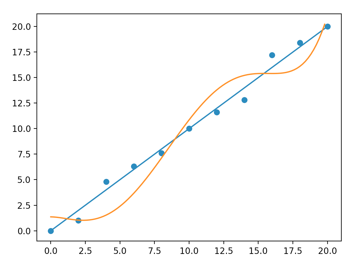
This leads us to a very important topic. When we increase the complexity of our model, we risk the chance of modeling the noise also. If we do not have enough sample data to cancel out the noise, we make bad predictions. But, even without the noise, we can still have a bad model. Let’s walk through an example below. We start with training samples with input values and output range from 0 to 20. How will you model an equation to link the data points below?

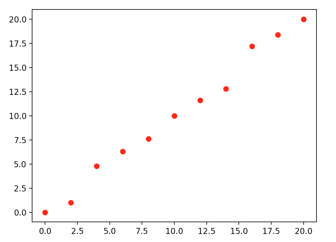
One possibility is \(y = x\) which is simple and just misses two points on the left and two on the right.

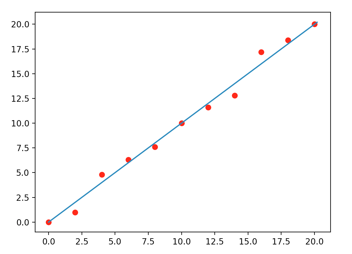
But, when we show it to our android Pieter, who has a much higher computational capability than us. He models it as:

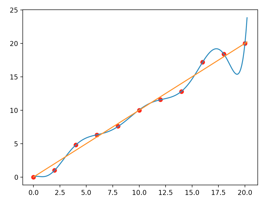
Which model is correct? The answer is “don’t know”. Someone thinks the first one is simpler, and simple explanations deserve more credit. But, if you show it to a stock broker, they may say the second curve looks closer to the market closing price of a stock. In general, we should ask whether our model is too “custom tailored” to the training dataset and fails to make generalized predictions. Even the second model fits the training data completely, but it can make poor predictions if the true model is proven to be a simple straight line.

When we have a complex model but not enough data, we can easily overfit the model which memorizes the training data but fails to make generalized predictions.

Validation

Machine learning is about making predictions. A model that has 100% accuracy in training can still be a bad model. To test the real performance, we split our data into three parts: say 80% for training, 10% for validation and 10% for testing. During training, we use the training dataset to build models with different hyperparameters. We run those models with the validation dataset and pick the one with the highest accuracy. This strategy works if the validation dataset is similar to what we want to predict. But, as a last safeguard, we use the 10% testing data for a final insanity check. This testing data is for a final verification, but not for model selection. If your testing result is dramatically different from the validation result, the data should be randomized more, or more data should be collected.

Validation data is used to select hyperparameters and models with the highest accuracy. The testing data should never use to select a model. It should be used very infrequently just for insanity check.

Visualization

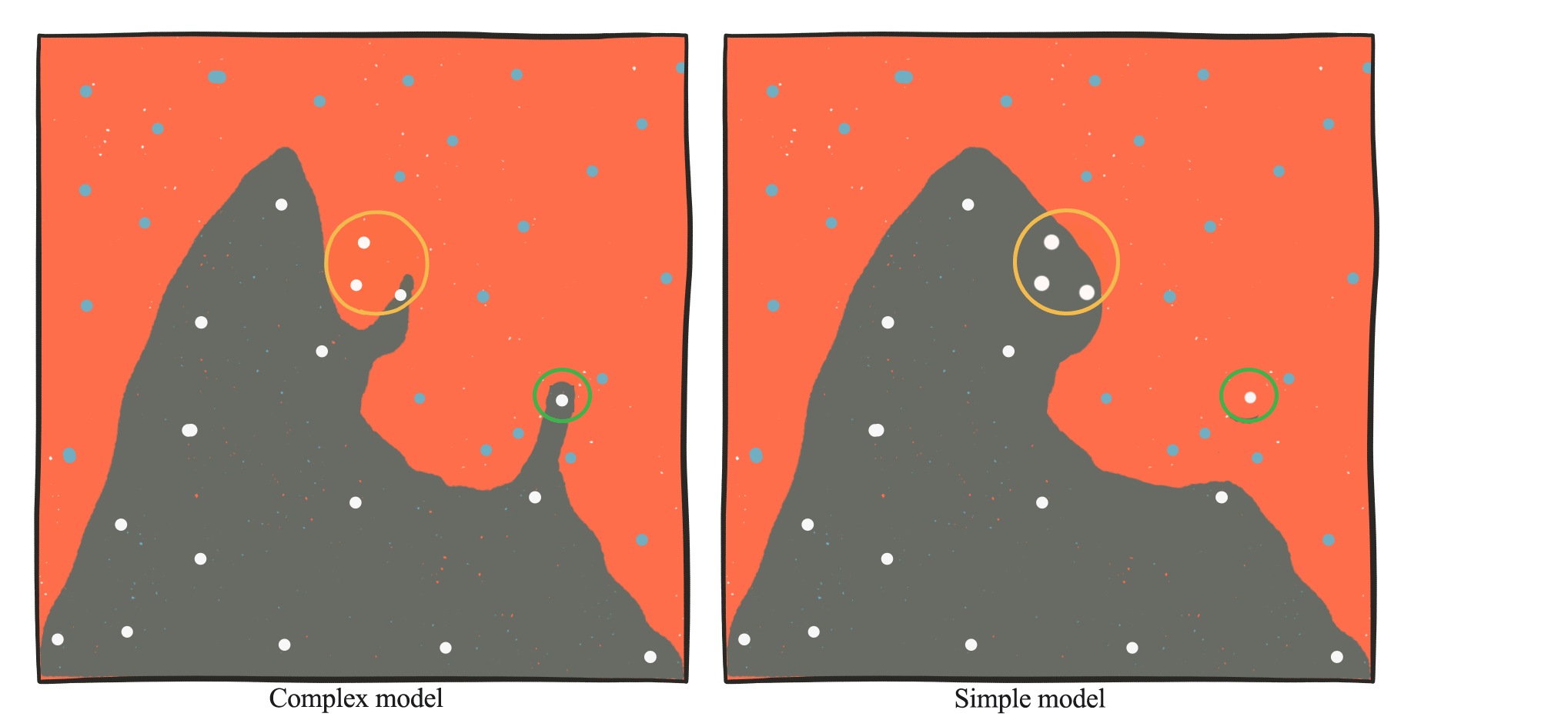
Let’s visualize some of the overfit problem. We can train a model to create a boundary to separate the blue dots from the white dots below. A complex model (the left picture) can produce ad hoc boundaries compared to a low complexity model. In the yellow-circled area, if the two left white dot samples is missing in our training dataset, a complex model may create an odd shaped boundary just to include this white dot. A low complexity model produces a smoother surface, which sometimes makes more generalized predictions. A complex model is vulnerable to outliers. For example, the white dot in the green circle may be incorrectly labeled as white. In a simple model, the boundary is much smoother and may simply ignore this outlier.

Recall from Pieter’s equation, our sample data can be modeled nicely with the following equations:

In fact, there are infinite solutions having different polynomial orders \(x^k\).

Compared with the linear model \(y = x\), the \(\| coefficient \|\) in Pieter’s equation is higher but it seems they are cancelling out each other. In addition, the higher the order, the harder to train the model because of the larger search space from the additional parameters. The expanded search space from the high polynomial order has very steep gradients that makes training even harder.

Let us create a polynomial model with order 5 to fit our sample data.

We need more iterations to train this model and it is less accurate than a model with order three.

So why don’t we focus on making a model with the right complexity. In real life problems, a complex model is the only way to push accuracy to an acceptable level. A better solution is to control overfitting rather than making the model simpler. One simple way is to add more training data such that it is much harder to overfit. Here, double our training data produces a model closer to a straight line. Unfortunately, labeling large training dataset in real problems can be expensive.

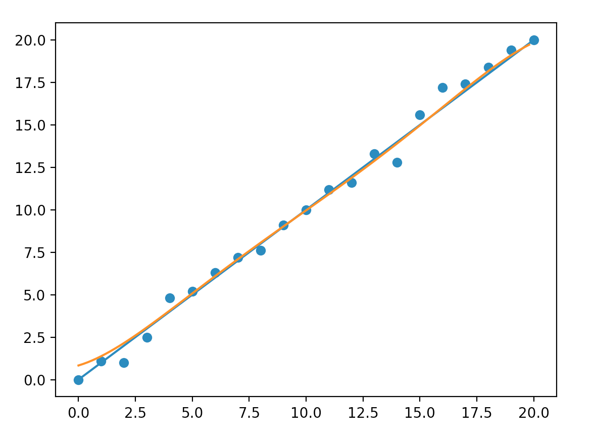
Complex models sometimes create ad hoc ways to fit training data that does not generalize. Increase the volume of training data reduces overfit effectively but can be expensive to do.

However, sometimes we can reduce the complexity of the model without sacrifice its accuracy. Complexity is proportional to the amount of parameters. We can remove features that can be directly or indirectly derived by others. We can design models that share parameters. In CNN, we reuse the same kernel parameters across spatial dimension. Because CNN is interested in detect a feature regardless of its spatial location, sharing kernels reduce the amount of parameters but not its power.

Regularization

Regularization punishes over-complexity. As we have observed before, there are many solutions to a DL problem. To have a close fit, however, the coefficient usually has a larger magnitude.

Overfit model tends to have larger magnitude. To avoid overfitting, we add a penalty in the cost function to penalize large magnitude. In this example, we use a L2 norm (L2 regularization) \(||W||\) as the penalty.

Penalize model complexity is called regularization. Here, we introduce another hyperparameter called regularization factor \(\lambda\) to penalize overfitting.

Regularization favors less complex model if the cost reduction from the complex model is less significant.

After many repetitions of trial, we pick \(\lambda\) to be 1. With the regularization, our model makes better predictions without adding extra training samples.

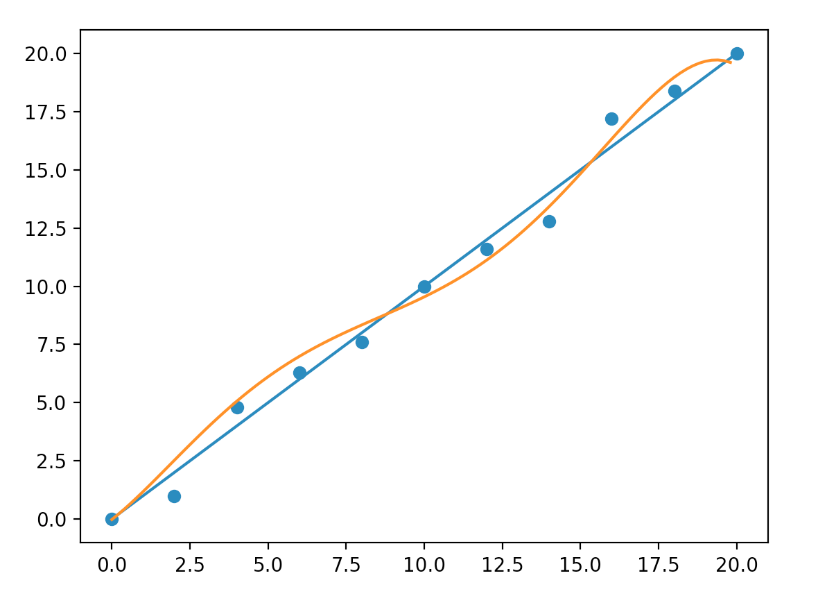
Like other hyperparameters, the selection process for \(\lambda\) is trial and error. In fact, we use a relatively high \(\lambda\) because there are only a few trainable parameters in the model. In real life problems, \(\lambda\) is much lower because the number of trainable parameters are usually in millions.

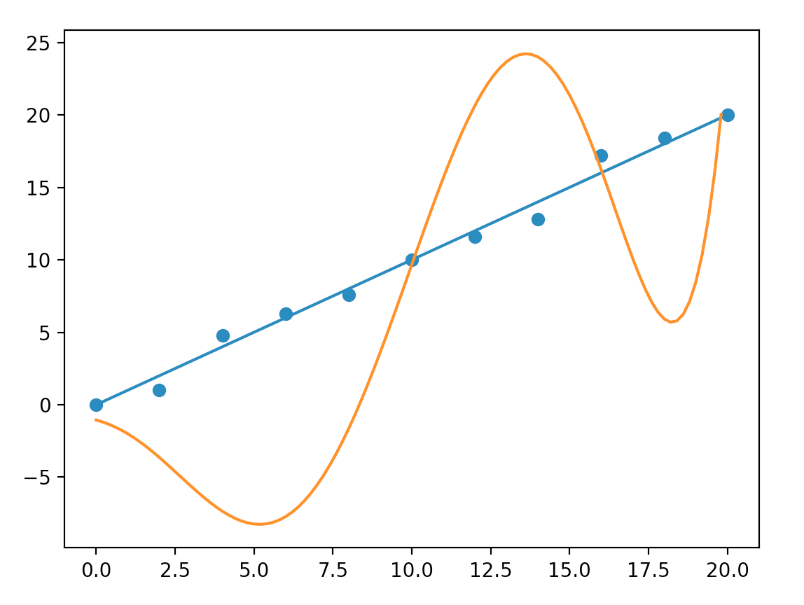
When we build our model, we try out a polynomial model with order of nine. Even after a long training, the model still makes poor predictions. We decide to start with a model with order of three and increase it gradually. This is another example to demonstrate why we should start with a simple model first. At seven, we find the model is too hard to train. The following is what a seven-order model predicts:

Classification

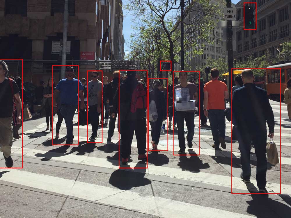
A very important part of deep learning is classification. We have mentioned object recognition before. These are classification problems asking the question: what is this? For example, for Android Pieter to safely walk in a street, he needs to learn what is a traffic light, and is there a pedestrian walking towards him. Classification applies to non-visual problems also. We classify whether an email is a spam or should we approve/disapprove a loan etc…

Like solving regression problem using DL, we use a deep network to compute a value. In classification, we call this a score. We apply a classifier to convert the score to a probability value between 0 and 1.

Logistic classifier

A score computed by a network takes on any value. A classifier squashes it to a probability value. For example, a binary classifier classifies whether an email is a spam or the medical test is positive, we apply a logistic function (also called a sigmoid function) to the score. If the output probability is lower than 0.5, we predict “no”, otherwise we predict “yes”.

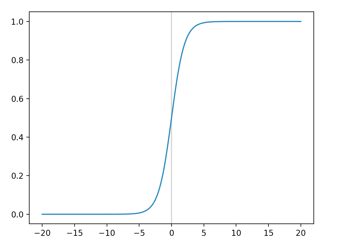
Softmax classifier

For many classification problems, we categorize an input to one of the many classes. For example, we can classify an image to one of the 100 possible object classes. We use a softmax classifier to compute K probabilities, one per class for an input image and the combined probabilities remains 1.

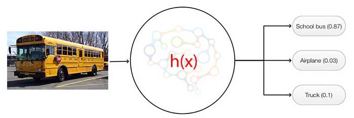
The network computes K scores per image. The probability that an image belongs to the class \(i\) will be.

For example, the school bus above may have a score of (3.2, 0.8, 0) for the class school bus, truck and airplane respectively. The probability for the corresponding class is

def softmax(z):
    z -= np.max(z)
    return np.exp(z) / np.sum(np.exp(z))

a = np.array([3.2, 0.8, 0])   # [ 0.88379809  0.08017635  0.03602556]
print(softmax(a))

To avoid the numerical stability problem caused by adding large exponential values, we subtract the inputs by its maximum. Adding or subtract a number from the input does not change the probability value in softmax.

z -= np.max(z)

logits is defined as a mean to measure odd.

If we combine the softmax equation with the logits equation, it is easy to see that the score is the logit.

That is why in many literatures and APIs, logit and score are interchangeable when a softmax classifier is used. However, other function’s output can be a logit. Sigmoid function output is also a logit.

Softmax is the most common classifier among others.

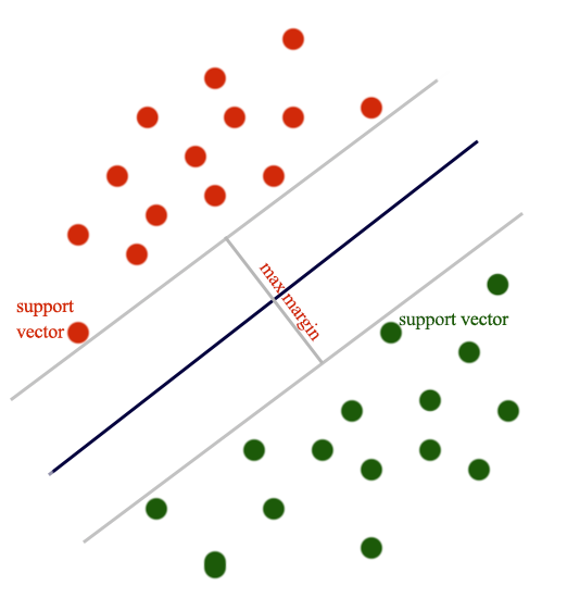
SVM classifier

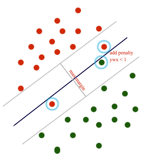
A SVM classifier uses the maximum margin loss (Hinge loss) and the L2-regularization as the cost function:

which \(y_i\) is the true label for datapoint \(i\). The class having the highest score will be the class predicted.

SVM classifier creates a boundary to separate classes with the largest possible margin.

The SVM loss (aka Hinge loss or Max margin loss) is defined as:

If the margin between the score of the true label and the score of a class is less than 1, we add it to the cost. Otherwise, add nothing. For example, with a score of (8, 14, 9.5, 10) for (class 1, class 2, class 3, class 4) and the true label is class 4. The SVM loss is:

We only penalize predictions that are in-correct or within a specific margin.

Softmax vs SVM

Softmax outputs probabilities which have better interpretations than scores in SVM. The value of a score has little interpretable values. SVM cares about the wrong predictions or predictions that are not too certain. Softmax penalizes all datapoints even their predictions are reasonably good (only penalize at a smaller extend). In practice, the performance between both are small.

Entropy

In DL, we often use the cross entropy or the KL-Divergence as our cost function. Those terms occurs frequently in research papers. In this section, we will understand what are they?

Entropy measures the amount of information. In data compression, it represents the minimum number of bits in representing data. By definition, entropy is defined as:

Suppose we have strings only composed of “a”, “b” or “c” with the chance of occurrence be 25%, 25% and 50% respectively. The entropy is:

We will use bit 0 to represent ‘c’ and bits 10 for ‘a’ and bits 11 for ‘b’. In average, we need 1.5 bits per character to represent a string.

Cross entropy

Cross entropy is defined as:

If entropy measures the minimum of bits to encode information using the most optimized scheme. Cross entropy measures the minimum of bits to encode \(y\) using the wrong optimized scheme from \(\hat{y}\). The cross entropy is always higher than entropy unless both distributions are the same: you need more bits to encode the information if you use a less optimized scheme.

In our previous example, we classify a picture as either a bus, a truck or an airplane. The output probability has the format: (bus, truck, airplane). The true label probability distribution for a bus is (1, 0, 0) and our model prediction can be (0.88, 0.08, 0.04).

The cross entropy of this example is:

KL Divergence

KL Divergence is defined as:

In machine learning, KL Divergence measures the difference between 2 probability distributions.

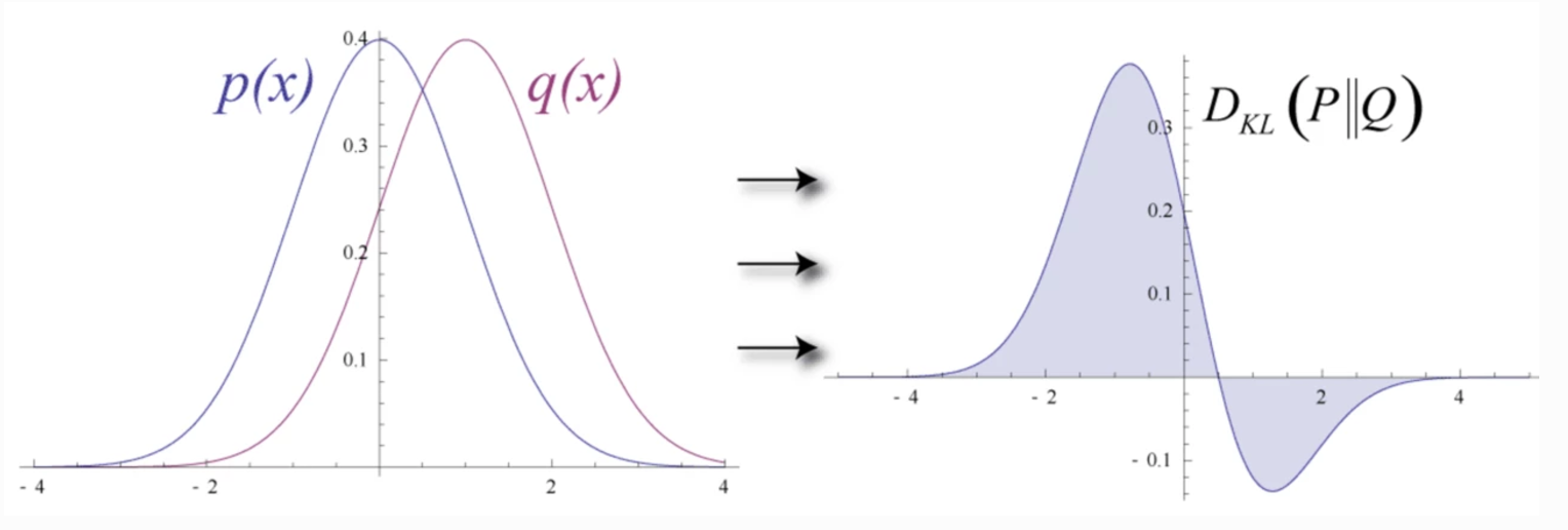
(Source Wikipedia)

It becomes a very good cost function to penalize the difference between the true labels and the predictions made by the model. It is even better for stochastic processes when the true label \(y_i\) is stochastic rather than deterministic (with probability either 0 or 1).

Solving cross entropy = solving KL-divergence

KL divergence is simply cross entropy \(H(y, \hat{y})\) minus entropy \(H(y)\) (the extra bits needed to encode the data):

The entropy of the true label is un-related with how we model it, i.e. \(\frac{\partial{H(y)}}{\partial{w}} = 0\). Therefore, the optimal solution for the KL-divergence is the same as that of the cross entropy.

Optimizing KL-divergence is the same as optimizing cross entropy.

KL-Divergence is more intuitive in the cost function discussion. In some research, we add constraints to KL-divergence to optimize our model. Nevertheless, cross entropy requires less computation than KL-divergence and used frequently in deep learning.

For a deterministic process, \(y_i\) is always equal to 1 for the true label and 0 otherwise. Hence, the cross entropy can be further simplified as:

Choice of cost function

Deep learning is about knowing your costs. Good cost function builds good models. San Francisco is about 400 miles from Los Angeles. It costs about $80 for the gas. When you order food from a restaurant, they do not deliver to homes more than a few miles away. From their perspective, the cost grows exponentially with distance. So in reality, we can modify our cost function to address special objectives. For example, some cost functions ignore outliers better than others.

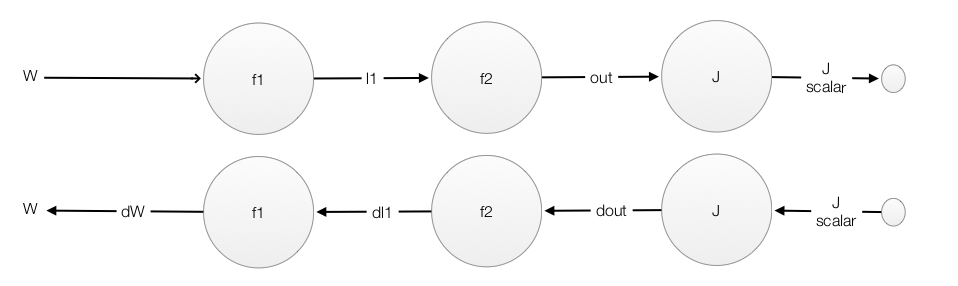
Mean square error (MSE)

We have used MSE for regression problems before. We can use MSE in classification. But, in practice, we use cross entropy loss instead. As demonstrated before, we learn very slowly when the node is saturated (when gradient is small). However, there is a way to solve this issue. Even the partial derivative of the sigmoid function in those regions is small but we can make \(\frac{\partial J}{\partial out}\) very large if the prediction is bad. The sigmoid function squashes values exponentially. We need a cost function that punishes bad predictions in the same scale to counter that. Squaring the error in MSE is not good enough. Cross entropy punishes bad predictions exponentially. That is why the cross entropy cost function trains better than MSE in the classification problems.

We pick cost functions easier to optimize and meet our objectives.

Deep learning network (Fully-connected layers) CIFAR-10

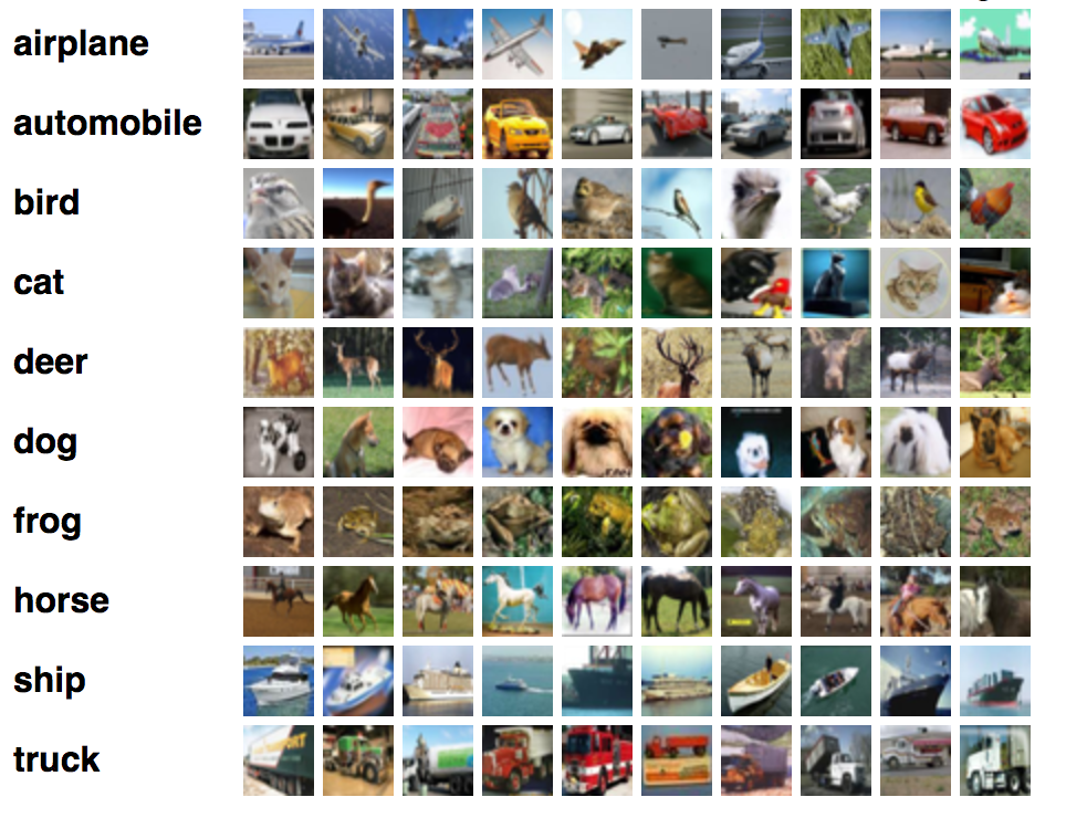
Let’s put together everything to solve the CIFRA-10. CIFAR-10 is a computer vision dataset for object classification. It has 60,000 32x32 color images belonging to one of 10 object classes, with 6000 images per class.

(Source Alex Krizhevsky)

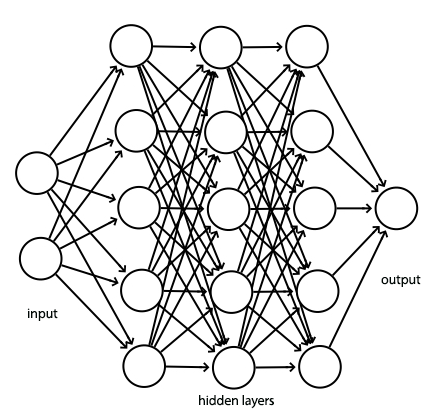
We implement a fully connected network similar to the following to classify the CIFRA images. In this implementation, we use a softmax classifier, L2 regularization and a cross entropy cost function.

Let’s repeat some boiler plate code that we did before. This is the forward feed and the back propagation code for \(y = Wx + b\) and the ReLU activation.

def affine_forward(x, w, b):
    out = x.reshape(x.shape[0], -1).dot(w) + b
    cache = (x, w, b)
    return out, cache

def affine_backward(dout, cache):
    x, w, b = cache
    dx = dout.dot(w.T).reshape(x.shape)
    dw = x.reshape(x.shape[0], -1).T.dot(dout)
    db = np.sum(dout, axis=0)
    return dx, dw, db

def relu_forward(x):
    out = np.maximum(0, x)
    cache = x
    return out, cache

def relu_backward(dout, cache):
    dx, x = None, cache
    dx = dout
    dx[x < 0] = 0
    return dx

We combine them to form a forward feed and a backpropagation “affine relu” layer. We will build our hidden layers with them:

def affine_relu_forward(x, w, b):
    a, fc_cache = affine_forward(x, w, b)
    out, relu_cache = relu_forward(a)
    cache = (fc_cache, relu_cache)
    return out, cache

def affine_relu_backward(dout, cache):
    fc_cache, relu_cache = cache
    da = relu_backward(dout, relu_cache)
    dx, dw, db = affine_backward(da, fc_cache)
    return dx, dw, db

We use a softmax classifier to compute the probabilities for each class. We subtract the score with its maximum value to improve numeric stability.

Since the true label distribution is 1 for the true value and zero otherwise, we computed the simplified cross entropy cost function as:

def softmax_loss(x, y):
    
    # Subtract from the max for better numeric stability.
    probs = np.exp(x - np.max(x, axis=1, keepdims=True)) 
    probs /= np.sum(probs, axis=1, keepdims=True)
    N = x.shape[0]
	
    # probs[np.arange(N), y] is the probability of the prediction 
    # for the true label class y.
    loss = -np.sum(np.log(probs[np.arange(N), y])) / N
    
    dx = probs.copy()
    dx[np.arange(N), y] -= 1
    dx /= N
    return loss, dx

We are creating a FullyConnectedNet network with 3 hidden layers with (100, 50, 25) nodes respectively. We also initialize \(w\) with a random normal distribution.

class FullyConnectedNet(object):

    def __init__(self, hidden_dims, input_dim=3 * 32 * 32, num_classes=10, reg=0.0,
                 weight_scale=1e-2, dtype=np.float32):
        self.reg = reg
        self.num_layers = 1 + len(hidden_dims)
        self.dtype = dtype
        self.params = {}

        layers = [input_dim] + hidden_dims + [num_classes]
        # Initialize the W & b for each layers 
        for i in range(self.num_layers):
            self.params['W%d' % (i + 1)] = np.random.randn(layers[i], layers[i + 1]) * weight_scale
            self.params['b%d' % (i + 1)] = np.zeros(layers[i + 1])

        # Cast all parameters to the correct datatype
        for k, v in self.params.iteritems():
            self.params[k] = v.astype(dtype)
			
			
model = FullyConnectedNet([100, 50, 25], weight_scale=5e-2, dtype=np.float64)			

The loss function is responsible for

• Process the forward feed.
• Call softmax_loss to compute the cross entropy loss and later add regularization cost.
• Process the backpropagation and compute the gradients.

Retrieve \(W\) & \(b\), and process the forward feed:

def loss(self, X, y=None):
    X = X.astype(self.dtype)
    # We reuse the same method for prediction. So we have the train mode and the test mode (make prediction.)
    mode = 'test' if y is None else 'train'

    layer = [None] * (1 + self.num_layers)
    cache_layer = [None] * (1 + self.num_layers)

    layer[0] = X

    # Feed forward for each layer define in FullyConnectedNet([100, 50, 25], ...)
    for i in range(1, self.num_layers):
        # Retrieve the W & b
        W = self.params['W%d' % i]
        b = self.params['b%d' % i]
        # Feed forward for one affine relu layer
        layer[i], cache_layer[i] = affine_relu_forward(layer[i - 1], W, b)

    last_W_name = 'W%d' % self.num_layers
    last_b_name = 'b%d' % self.num_layers
    # From the last hidden layer to the output layer, we do an affine op but not ReLU
    scores, cache_scores = affine_forward(layer[self.num_layers - 1],
                                          self.params[last_W_name],
                                          self.params[last_b_name])

    # If just making prediction, we return the scores										  
    if mode == 'test':
        return scores
    ...

Then we call softmax_loss to compute the cross entropy loss and add L2 regularization.

def loss(self, X, y=None):
    ...
	
    loss, grads = 0.0, {}
    # Compute the loss
    loss, dscores = softmax_loss(scores, y)

    # For each layer, add the regularization loss
    for i in range(self.num_layers):
        loss += 0.5 * self.reg * np.sum(self.params['W%d' % (i + 1)] ** 2)

    ...

Finally, we compute the gradients using the backpropagation.

def loss(self, X, y=None):
    ...
	
    # Back progagation the output to the last hidden layer
    dx = [None] * (1 + self.num_layers)
    dx[self.num_layers], grads[last_W_name], grads[last_b_name] = affine_backward(dscores, cache_scores)
    grads[last_W_name] += self.reg * self.params[last_W_name]

    # Back progagation from the last hidden layer to the first hidden layer
    for i in reversed(range(1, self.num_layers)):
        dx[i], grads['W%d' % i], grads['b%d' % i] = affine_relu_backward(dx[i + 1], cache_layer[i])
        grads['W%d' % i] += self.reg * self.params['W%d' % i]

    return loss, grads

Here is the code of training the model. FullyConnectedNet builds the model. Solver takes the model and the training data. It iterates the training data in 10 epochs. The model’s loss function will be called to calculate the gradients and an Adam optimizer will update \(W\) and \(b\). Adam optimizer is a gradient descent optimizer heavily used in deep learning. (We will cover this in a later section.) We rarely need to write the Solver ourself since most deep learning platforms will provide those services. Since the basic coding on parameter update is already cover, we will not repeat here again.

model = FullyConnectedNet([100, 50, 25],
              weight_scale=weight_scale, dtype=np.float64)
solver = Solver(model, data,
                print_every=100, num_epochs=10, batch_size=200,
                update_rule='adam',
                optim_config={
                  'learning_rate': learning_rate,
                }
         )
solver.train()

After the model is trained, we want to compute the accuracy for both validation and testing dataset.

X_test, y_test, X_val, y_val = data['X_test'], data['y_test'], data['X_val'], data['y_val']

y_test_pred = np.argmax(model.loss(X_test), axis=1)
y_val_pred = np.argmax(model.loss(X_val), axis=1)
print('Validation set accuracy: ', (y_val_pred == y_val).mean())
print('Test set accuracy: ', (y_test_pred == y_test).mean())

This model will achieve 50+% accuracy far better than a random guess (10% accuracy).

Deep learning is about creating a model by learning from data. We have solved a visual recognition problem that is otherwise difficult to solve. Instead of coding all the rules, which is impossible for the CIFRA problem, we create a FC network to learn the model from data. The accuracy can be further improved to 90+% by adding convolution layer (CNN) on top of the FC network. CNN will be covered in a separate article but we will continue to study the basic building block for deep learning first.

MNist

One of the first deep learning datasets that most people learn is the MNist. It is a dataset for handwritten numbers from 0 to 9.

We will implement code using the TensorFlow to solve the problem with 98+% accuracy. TensorFlow is a deep learning software platfrom from Google. It provides higher level APIs to build and train model much easier.

Unlike the code with numpy, TensorFlow constructs a graph describing the network first. Here, we declare a placeholder for our input features (the pixel values of the image) and the labels. The real data will be provided later in the execution phase.

x = tf.placeholder(tf.float32, [None, 784])
labels = tf.placeholder(tf.float32, [None, 10])  # True label.

We declare \(W\) and \(b\) as variables. Those are trainable variables that we want to learn from the training dataset. In the declaration, we also declare the method to initialize the variables. Remember that all computations include initialization are delayed until the execution phase later.

W1 = tf.Variable(tf.truncated_normal([784, 256], stddev=np.sqrt(2.0 / 784)))
b1 = tf.Variable(tf.zeros([256]))
W2 = tf.Variable(tf.truncated_normal([256, 100], stddev=np.sqrt(2.0 / 256)))
b2 = tf.Variable(tf.zeros([100]))
W3 = tf.Variable(tf.truncated_normal([100, 10], stddev=np.sqrt(2.0 / 100)))
b3 = tf.Variable(tf.zeros([10]))

We define 2 hidden layers. Each has a matrix multiplication operation followed by ReLU. Then we define an output layer with the matrix multiplication only.

### Building a model
# Create a fully connected network with 2 hidden layers
# 2 hidden layers using relu (z = max(0, x)) as an activation function.
h1 = tf.nn.relu(tf.matmul(x, W1) + b1)
h2 = tf.nn.relu(tf.matmul(h1, W2) + b2)
y = tf.matmul(h2, W3) + b3

Now, we define our loss function: a cross entropy cost plus a L2 regularization penalty. We use an Adam optimizer (named as train_step) to perform the gradient descent to optimize \(W\). We also have a placeholder for \(\lambda\) so a user can tune the regularization later.

# Cost function & optimizer
# Use a cross entropy cost fuction with a L2 regularization.
lmbda = tf.placeholder(tf.float32)

cross_entropy = tf.reduce_mean(
    tf.nn.softmax_cross_entropy_with_logits(labels=labels, logits=y) +
        lmbda * (tf.nn.l2_loss(W1) + tf.nn.l2_loss(W2) + tf.nn.l2_loss(W3)))
		
train_step = tf.train.AdamOptimizer(learning_rate=0.001).minimize(cross_entropy)

Once the declaration is completed, we create a session to execute the graph and train the network for 10,000 iterations. For each iteration, we retrieve the next batch of the training data and execute the Adam optimizer “train_step”.

# Create an operation to initialize the variable
init = tf.global_variables_initializer()
# Now we create a session to execute the operations.
with tf.Session() as sess:
    sess.run(init)
    # Train
    for _ in range(10000):
      batch_xs, batch_ys = mnist.train.next_batch(100)
      sess.run(train_step, feed_dict={x: batch_xs, labels: batch_ys, lmbda:5e-5})

Once the training is completed, we create another operation accuracy to compute the accuracy of our model.

with tf.Session() as sess:
    ...
	
    # Test trained model
    correct_prediction = tf.equal(tf.argmax(y, 1), tf.argmax(labels, 1))
    accuracy = tf.reduce_mean(tf.cast(correct_prediction, tf.float32))

Then we run the accuracy operation with our testing dataset and print out the results.

with tf.Session() as sess:
    ...
	
    print(sess.run(accuracy, feed_dict={x: mnist.test.images,
                                          labels: mnist.test.labels}))

For completeness, here is the full code listing. This file depends on “tensorflow.examples.tutorials.mnist” which reads the MNist data.

import argparse
import sys

from tensorflow.examples.tutorials.mnist import input_data

import tensorflow as tf
import numpy as np

FLAGS = None


def main(_):
  # Import data
  mnist = input_data.read_data_sets(FLAGS.data_dir, one_hot=True)

  ### Building a model
  # Create a fully connected network with 2 hidden layers
  # Initialize the weight with a normal distribution.
  x = tf.placeholder(tf.float32, [None, 784])
  labels = tf.placeholder(tf.float32, [None, 10])  # True label.
  
  W1 = tf.Variable(tf.truncated_normal([784, 256], stddev=np.sqrt(2.0 / 784)))
  b1 = tf.Variable(tf.zeros([256]))
  W2 = tf.Variable(tf.truncated_normal([256, 100], stddev=np.sqrt(2.0 / 256)))
  b2 = tf.Variable(tf.zeros([100]))
  W3 = tf.Variable(tf.truncated_normal([100, 10], stddev=np.sqrt(2.0 / 100)))
  b3 = tf.Variable(tf.zeros([10]))


  # 2 hidden layers using relu (z = max(0, x)) as an activation function.
  h1 = tf.nn.relu(tf.matmul(x, W1) + b1)
  h2 = tf.nn.relu(tf.matmul(h1, W2) + b2)
  y = tf.matmul(h2, W3) + b3

  # Cost function & optimizer
  # Use a cross entropy cost fuction with a L2 regularization.
  lmbda = tf.placeholder(tf.float32)
  cross_entropy = tf.reduce_mean(
      tf.nn.softmax_cross_entropy_with_logits(labels=labels, logits=y) +
         lmbda * (tf.nn.l2_loss(W1) + tf.nn.l2_loss(W2) + tf.nn.l2_loss(W3)))
  train_step = tf.train.AdamOptimizer(learning_rate=0.001).minimize(cross_entropy)

  init = tf.global_variables_initializer()
  with tf.Session() as sess:
      sess.run(init)
      # Train
      for _ in range(10000):
        batch_xs, batch_ys = mnist.train.next_batch(100)
        sess.run(train_step, feed_dict={x: batch_xs, labels: batch_ys, lmbda:5e-5})

      # Test trained model
      correct_prediction = tf.equal(tf.argmax(y, 1), tf.argmax(labels, 1))
      accuracy = tf.reduce_mean(tf.cast(correct_prediction, tf.float32))
      print(sess.run(accuracy, feed_dict={x: mnist.test.images,
                                          labels: mnist.test.labels}))

if __name__ == '__main__':
  parser = argparse.ArgumentParser()
  parser.add_argument('--data_dir', type=str, default='/tmp/tensorflow/mnist/input_data',
                      help='Directory for storing input data')
  FLAGS, unparsed = parser.parse_known_args()
  tf.app.run(main=main, argv=[sys.argv[0]] + unparsed)

# 0.9816

This code demonstrates the power to solve a complex visual problem with few lines of DL code. In fact, there are higher level TensorFlow APIs that can even make the code smaller. With 10,000 iterations, our model achieved an accuracy above 98%.

Weight initialization

Proper weight initialization is critical. This is a common cause when the model performs no better than random guess. Often, people accidentally initialize \(W\) with 0s. This is like every nodes are dead and loss signal cannot be backpropagated. We want some non-symmetry on \(W\): not similar values for every nodes. So nodes can learn different features. We initialize \(W\) with a Gaussian distribution with \(\mu = 0\). We do not want \(W\) to have large magnitude which will fall into saturated area where gradient is small and therefore learning is slow.

Let’s generate 20,000 values of \(W\) with \(\mu = 0\) and \(\sigma^2 = 1\). Here is the distribution of \(W\).

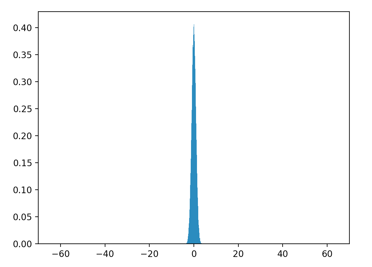
Let’s create a node with 1000 input. We initialize half of the \(x\) as 1 and the other half as 0. We generate 20,000 output with.

The variance of the output jumps almost 500 times and the plot is almost flat.

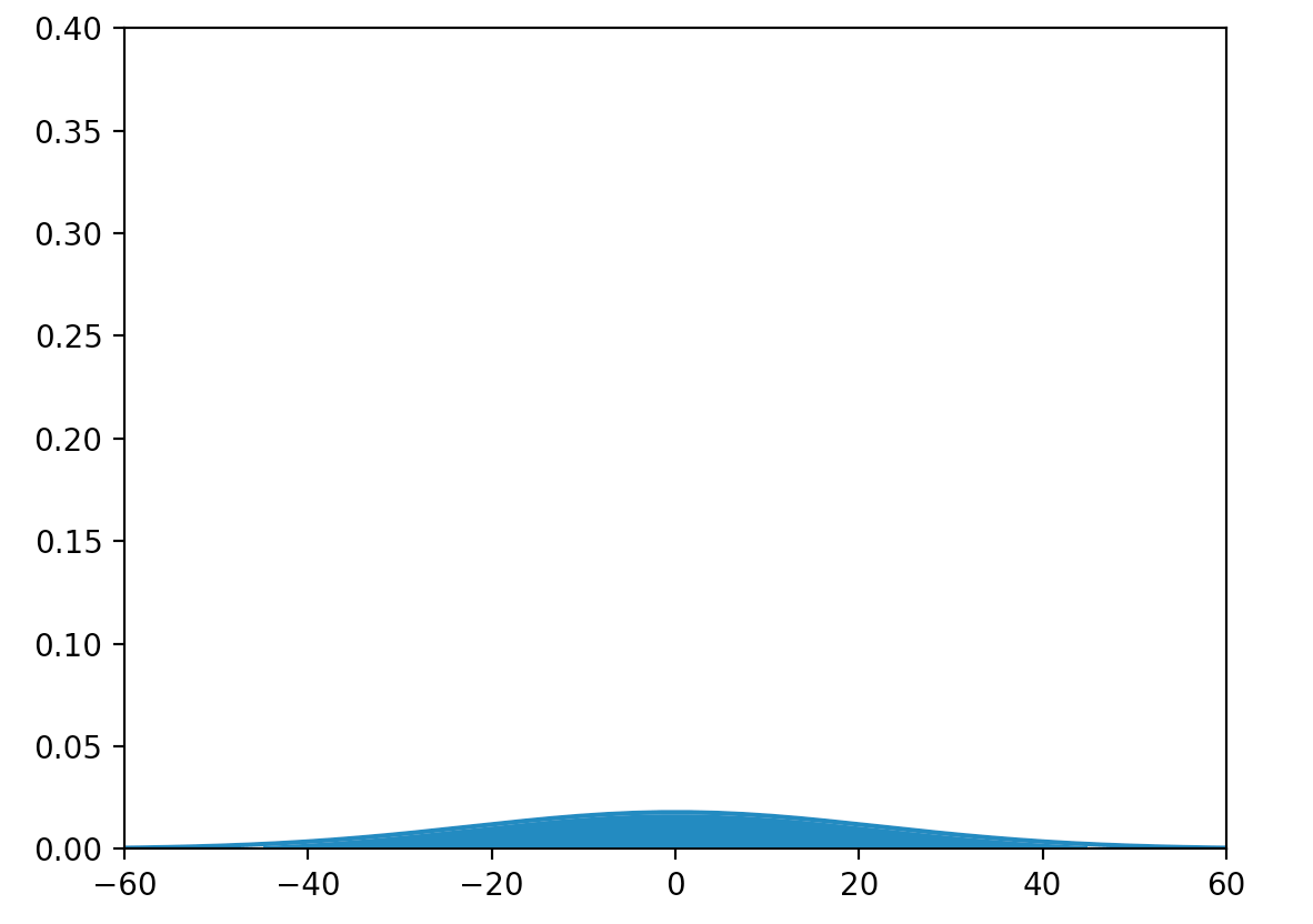
If we feed this output into the activation function. Huge portion of the values are in the saturation region for any activation functions we discussed as far. So what is the \(\sigma\) value we should use to generate \(W\)?

Hence, if we want the input to the activation function to have \(\mu = 0\) and \(\sigma^2 = 1\), we need to scale \(w\) by \(\frac{1}{\sqrt{n}}\). With ReLU activation, we want to scale it with

w = np.random.randn(n) * sqrt(2.0/n)

Training parameters

Weight decay

We updates \(W\) by

When we add a L2-normalization,

It effectively performs a weight decay:

Rate of decay

To maintain a constant learning rate is not a good idea. In later phase, we want much smaller steps to avoid oscillation. After some initial training, we can start decaying the learning rate for every N iterations. For example, after 10,000 iterations, the learning rate will be decreased by a factor for every 20,000 iterations:

where decay factor is another hyperparameter say 0.95.

Momentum update

We mentioned that gradient descent is like dropping a ball in a bowl. But our gradient descent adjusts the parameters by the gradient of the current location of \(W\) only. In the physical world, the movement of the ball depends on the location and also on the momentum of the ball. We could adjust \(W\) by the gradient and its history rather than throwing all the history away. If we recall the stochastic gradient descent, it follows a zip zap pattern rather than a smooth curve. With this historical information, we can make stochastic gradient or mini-batch gradient to behave more smoothly.

Here we introduce a variable \(v\), which behaves like the momentum in the physical world. In each iteration, we update \(v\) by keeping a portion of v minus the change caused by the gradient at current location. \(mu\) controls how much history information to keep, and this will be another hyperparameter. Researchers may describe \(mu\) as fraction. If you recall the oscillation problem before, this actually becomes a damper to stop the oscillations. Momentum based gradient descent often has a smoother path and settles to a minimum closer and faster.

v = mu * v - learning_rate * dw
w += v

Nesterov Momentum

In Momentum update, we use the current location of \(w\) to compute \(dw\). In Nesterov Momentum, the current location is replaced with a look-ahead location: the location where the ball should go without taking the current location into account. Nesterov Momentum converges better than Momentum update.

In the program below, instead of using location \(w\) to compute \(dw\), we use location \(w_{ahead}\) to compute \(dw\).

w_ahead = w + mu * v
v = mu * v - learning_rate * dw_ahead
w += v

In practice, people use the following formula:

v_prev = v
v = mu * v - learning_rate * dw 
w += -mu * v_prev + (1 + mu) * v 

Adagrad

If the input features are not scaled correctly, it is impossible to find the right learning rate that works for all the features. This indicates the learning rate needs to be self-adapted for each tunable parameter. One way to do it is to remember how much change has made to a specific \(W_i\). We should reduce the rate of change for parameters that already have many updates. This mitigates the oscillation problem because it acts like a damper again. In Adagrad, we reduce the learning rate with a ratio inversely proportional to the L2 norm of all previous gradients \(dw_i\).

cache += dw**2
# add a tiny value to avoid division by 0.
w += - learning_rate * dw / (np.sqrt(cache) + 1e-7) 

Parameter based methods like Adagrad reduce the learning rate for parameters according to their accumulated changes.

RMSprop

Like Adagrad, RMSprop adjusts the learning rate according to the history of the gradients. But it uses a slightly different formular with the introduction of another hyperparameter decay_rate.

cache = decay_rate * cache + (1 - decay_rate) * dw**2
w += - learning_rate * dx / (np.sqrt(cache) + 1e-7)

RMSprop behaves like Adagrad but have mechanism to forget older changes.

Adam

Adam combines the concepts of momentum with RMSprop:

m = beta1*m + (1-beta1)*dw
v = beta2*v + (1-beta2)*(dw**2)
w += - learning_rate * m / (np.sqrt(v) + 1e-7)

Adam combines both momentum and parameter based gradient descent. Adam is the most often used method now.

Here is an example of using Adam Optimizer in TensorFlow

loss = tf.reduce_mean(
        tf.nn.softmax_cross_entropy_with_logits(labels=tf_train_labels, logits=logits)) \
           + lmbda * tf.nn.l2_loss(weights1) + lmbda * tf.nn.l2_loss(weights2) \
           + lmbda * tf.nn.l2_loss(weights3) + lmbda * tf.nn.l2_loss(weights4)

optimizer = tf.train.AdamOptimizer(0.0005).minimize(loss)

...

with tf.Session(graph=graph) as session:
    ...
    for step in range(num_steps):
        ...
        _, l, predictions = session.run(
            [optimizer], feed_dict=feed_dict)

Visualization of Gradient descent methods

Here are some animations produced by Alec Radford in demonstrating how the gradient descent behaves for different algorithms. Regular gradient descent (red) learns the slowest. Momentum based algorithm has a tendency to overshoot the target initially. Adagrad learns faster initially than RMSprop. But RMSprop provides a mechanism to erase old history which make learning more adaptable later.

Feature Scaling (normalization)

As discussed before, we want the feature input to be scaled correctly (normalized). If the features do not have similar scale, it will be hard for the gradient descent to work: the training parameters oscillate like the red arrow.

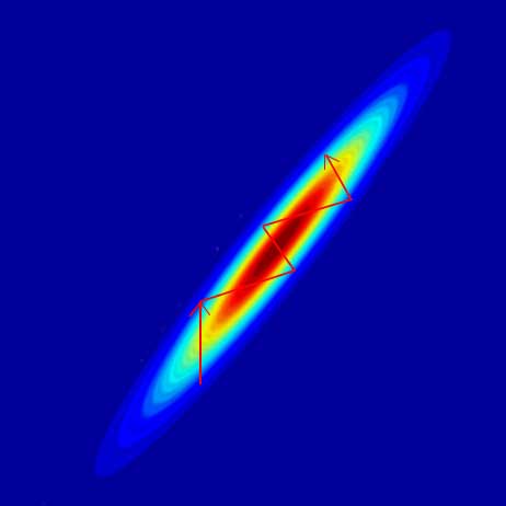
For example, with 2 input features, we want the shape to be as close to a circle as possible.

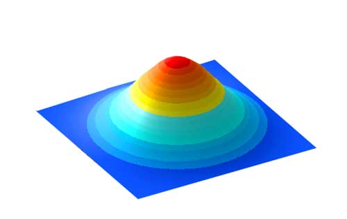
To achieve that we normalize the features in the dataset to have zero mean and unit variance.

For images, we normalize every pixel independently. We compute a mean and a variance at each pixel location for the entire training dataset. Therefore, for an image with NxN pixels, we use NxN means and variances to normalize the image.

In practice, we do not read all the training data at once to compute the mean or variance. We compute a running mean during the training. Here is the formula for the running mean:

where \(k\) is a small constant.

Use the running mean and variance from training dataset to normalize validation and testing data.

Whitening

In machine learning, we can train a model faster if features are not correlated (whitened). In a dating application, someone may prefer a tall person but not too thin. If we rescale the weight and height independent of each other, the rescaled features are still co-related. From the rescaled weight, we can tell easily whether a person is heavier than the average population. But usually, we are more interested to know whether the person is thinner in the same height group which is very hard to tell from the rescaled weight alone.

We can express the co-relations between features \(x_i\) and \(x_{j}\) in a covariance matrix:

Which \(E\) is the expected value.

Consider 2 data samples (10, 20) and (32, 52). The mean of \(x_1\) is \(\mu_1 = \frac {10+32}{2} = 21\) and \(\mu_2 = 36\)

The expected value of the first element in the second row will be:

From the covariance matrix \(\sum\), we can find a matrix \(W\) to convert \(x\) to \(x^{'}\) whose features are un-correlated with each other. For example, the contour plotting on the left below indicates weight and height are correlated (weight increase with height). On the right, the features are whitened with their correlation-ship recalibrate (taken out). For example, if the new \(weight^{'}\) feature is smaller than 0, we know the person is thinner in the same height group.

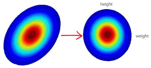
Whitening un-correlates features that make training more effective.

This sounds complicated, but can be done easily by Numpy linear algebra library.

X -= np.mean(X, axis = 0)    
cov = np.dot(X.T, X) / X.shape[0]

U,S,V = np.linalg.svd(cov)
Xdecorelate = np.dot(X, U)
Xwhite = Xdecorelate / np.sqrt(S + 1e-5)

Image data usually require 0 centered but does not require whitening.

Batch normalization

We have emphasized so many times the benefits of having features with mean = 0 and \(\sigma^2=1\)

But, why do we stop at the input layer only. Batch normalization renormalizes a layer output. For example, we renormalized the output of the affine layer (matrix multiplication) before feeding it into the ReLU.

def affine_batchnorm_relu_forward(x, w, b, gamma, beta, bn_param):
  h, h_cache = affine_forward(x, w, b)
  norm, norm_cache = batchnorm_forward(h, gamma, beta, bn_param)
  relu, relu_cache = relu_forward(norm)
  cache = (h_cache, norm_cache, relu_cache)
  return relu, cache

We apply the normalization formula below:

For a feature map with 100 elements, we compute 100 means and 100 variance from the batch samples. For example, if the batch size is 16, the mean for element \(i\) is computed by:

We feed \(z\) to a linear equation with the trainable scalar values \(\gamma\) and \(\beta\) (1 pair for each normalized layer).

The normalization can be undone if \(gamma = \sigma\) and \(\beta = \mu\). We initialize \(\gamma = 1\) and \(\beta =0\), so the input is normalized and therefore learns faster, and the parameters will be learned during the training.

def batchnorm_forward(x, gamma, beta, bn_param):
    sample_mean = np.mean(x, axis=0)
    sample_var = np.var(x, axis=0)

    sqrt_var = np.sqrt(sample_var + eps)
    xmu = (x - sample_mean)
    xhat = xmu / sqrt_var

    out = gamma * xhat + beta

Batch normalization solves a problem called internal covariate shift. As weights are updated, the distribution of outputs at each layer changes. With many deep layers, the distribution is not normalized even we start from a normalized input. Batch normalization normalized data at each layer again. So the gradient descent can train the model faster and more accurate. As a side bonus, we can increase the learning rate higher without lower the accuracy. Batch normalization also help regularize \(W\).

In the training, we use the mean and variance of the current training sample. But for testing, we do not use the mean/variance of the testing data. Instead, we record a running mean & variance during the training and apply it in validation or testing.

running_mean = momentum * running_mean + (1 - momentum) * sample_mean
running_var = momentum * running_var + (1 - momentum) * sample_var

We use this running mean and variance to normalize our testing data.

xhat = (x - running_mean) / np.sqrt(running_var + eps)
out = gamma * xhat + beta

Batch normalization is common practice to use before or after the activation functions including CNN layers.

This is the code to implement batch normalization in TensorFlow:

w_bn = tf.Variable(w_initial)
z_bn = tf.matmul(x, w_bn)

bn_mean, bn_var = tf.nn.moments(z_bn, [0])
scale = tf.Variable(tf.ones([100]))
beta = tf.Variable(tf.zeros([100]))

bn_layer = tf.nn.batch_normalization(z_bn, bn_mean, bn_var, beta, scale, 1e-3)
l_bn = tf.nn.relu(bn_layer)

Diminishing and exploding gradient

Cannot train a model if gradients explode or diminish. Monitoring gradients and \(\Delta W\) are very important in trouble shooting. In the following log, the gradient diminishes from the right layer (layer 6) to the left layer (layer 0). Layer 0 almost learns nothing.

iteration 0: loss=553.5
layer 0: gradient = 2.337481559834108e-05
layer 1: gradient = 0.00010808796151264163
layer 2: gradient = 0.0012733936924033608
layer 3: gradient = 0.01758514040640722
layer 4: gradient = 0.20165907211476816
layer 5: gradient = 3.3937365923146308
layer 6: gradient = 49.335409914253
iteration 1000: loss=170.4
layer 0: gradient = 0.0005143399278199742
layer 1: gradient = 0.0031069449720360883
layer 2: gradient = 0.03744160389724748
layer 3: gradient = 0.7458109132993136
layer 4: gradient = 5.552521662655173
layer 5: gradient = 16.857110777922465
layer 6: gradient = 37.77102597043024
iteration 2000: loss=75.93
layer 0: gradient = 4.881626633589997e-05
layer 1: gradient = 0.0015526594728625706
layer 2: gradient = 0.01648262093048127
layer 3: gradient = 0.35776408953278077
layer 4: gradient = 1.6930852548061421
layer 5: gradient = 4.064949014764085
layer 6: gradient = 12.7578637206897

Many deep networks suffer from this gradient diminishing problem. Let’s come back to backpropagation to understand the problems.

The gradient descent is computed as:

As indicated, the gradient descent depends on the loss \(\frac{\partial J}{\partial l_1}\) as well as the gradients \(\frac{\partial l_{k+1}}{\partial l_{k}}, \frac{\partial l_{k}}{\partial l_{k-1}} \dots\). Let’s look at a sigmoid activation function. If \(x\) is higher than 5 or smaller than -5, the gradient is close to 0. Hence, in these region, \(\frac{\partial l_{k}}{\partial l_{k-1}}\) is near zero and these node learns close to nothing regardless of the loss.

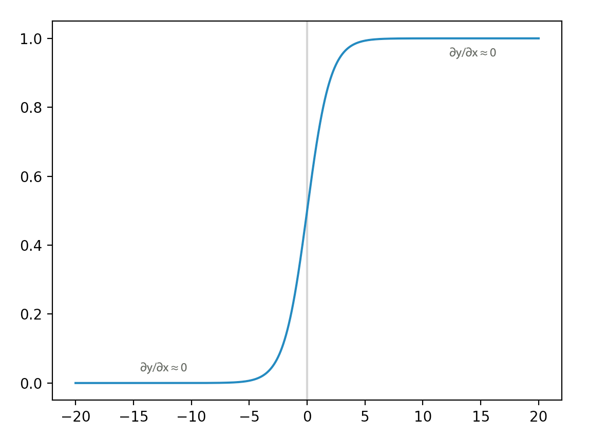
The derivative of a sigmoid function behaves like a gate to the loss signal. If the input is > 5 or <-5, it blocks most of the loss signal to propagate backwards. So, nodes on its left side layers learn little.

The deeper the networks, the more non-linearity and it makes gradient-based methods less efficient. (each layer composes more non-linearity on top of the previous ones)

In addition, the chain rule in the gradient descent has a multiplication effect. If we multiple numbers smaller than one, it diminishes quickly. On the contrary, if we multiple numbers greater than one, it explodes.

x

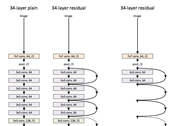
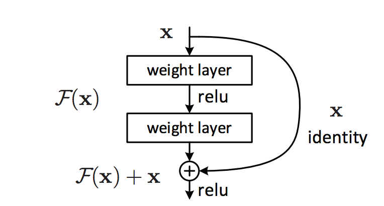
These problems happen more frequently for networks with very deep layers. Natural language networks use a looping layers with sharing parameters. Hence, their gradients may move in the same direction together, and vulnerable to these problems. To solve it, we have designed new computation nodes that can bypass an individual layer. Microsoft Resnet has 152 layers. Instead of backpropagate the cost through a long chain of nodes, Resnet have both pathways to backpropagate it through the convolution layer or by-passed through the arc. (Source Kaiming He, Xiangyu Zhang … etc)

Let’s demonstrate it with a node called LSTM that used in the natural language processing (NLP). In LSTM, the state of a cell is updated by

If we want to bypass this node such that the input \(C_{t-1}\) becomes the output \(C_t\), we just need to set \(gate_ {forget}=1\) and \(gate_{input} = 0\). So one way to address the diminishing gradient problem is to design a computation node with pathway that can bypass a node. At the beginning of the training, we initialize \(gate\) to bypass most nodes but have the network to learn the proper value for \(gate_ {forget}\) and \(gate_{input}\) eventually.

Diminish gradient can be mitigated by designing computation nodes that providing a bypassing pathway for the node.

Gradient clipping for gradient explosion

To avoid gradient explosion, we can apply gradient clipping to restrict values of the gradient. Gradient explosion happens more often in NLP.

In the example below, we use TensorFlow (a popular deep learning platform from Google) to clip the gradient if it is too big.

params = tf.trainable_variables()
opt = tf.train.GradientDescentOptimizer(learning_rate)
for b in xrange(time_steps):
    gradients = tf.gradients(losses[b], params)
    clipped_gradients, norm = tf.clip_by_global_norm(gradients, 5.0)

The gradients are rescaled according to the ratio \(\frac{5}{max(\| gradient \|, \| global \text{ } gradients \|)}\)

# t is each individual gradient
# global_norm is the norm for all gradients
# clip_norm is set to 5.0
global_norm = sqrt(sum([l2norm(t)**2 for t in t_list]))
t_list[i] * clip_norm / max(global_norm, clip_norm)

Dead nodes in gradient diminishing

The most effective method to resolve gradient diminishing in deep networks is layers bypassing.

ReLU remains the most popular activation functions. However, if there are too many dead nodes (activation=0), we can experiment leaky ReLU or other more advance activation functions like Maxout. In ReLU, \(y = max(0, Wx+b)\). In Maxout, we maintain 2 set of \(W\)s and \(b\)s. the output is computed as: \(y = max(W_1x+b_1, W_2x+b_2)\).

L0, L1, L2 regularization

Large W tends to overfit a model. L2 regularization adds the L2 norm to a cost function to reduce overfit.

Beside L2 norm, we can use L0 or L1 norm.

L0 regularization

L1 regularization

Comparison among L0, L1 and L2 regularization

The derivative of L2 norm is easy to compute and it is smooth which works well with gradient descent. Hence L2 regularization is very popular. \(W^*_b\) is the optimal \(W\) without the regularization. By adding the L2 regularization (the circle), we shift the optimal point \(W^*\) closer to 0.

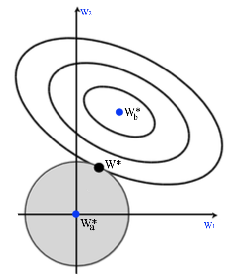
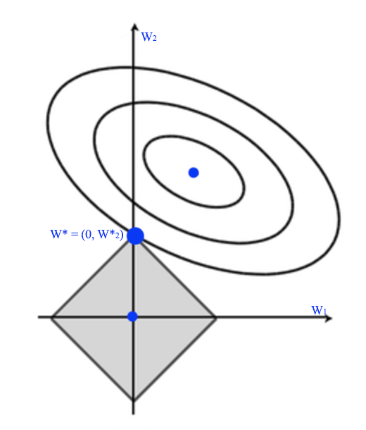
The shape of the L1 regularization is a rotated square instead of a circle since regularization cost is measured as \(\vert W \vert\) but not \(\| W \|\). L1 regularization tries to push some \(W^*_i\) to zero rather than closer to 0. So it increase the sparsity of \(w\).

L0 regularization adds a constant cost to the regular cost (blue curve) except at \(w=0\). The green curve is the new cost which have a sudden drop at 0 to to the green dot. Therefore, it can push more \(w\) to 0 comparing to L1 regularization.

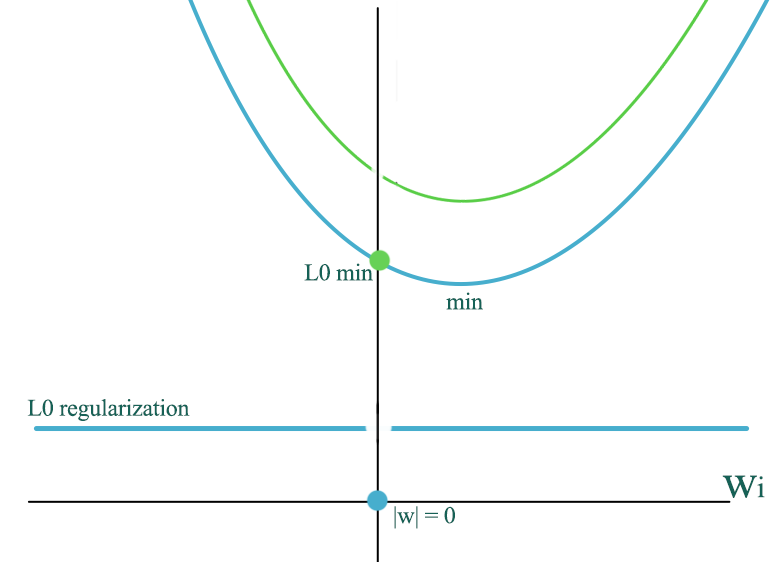
L1 and L0 regularization promotes sparsity for \(w\) which can be desirable to avoid overfitting when we have too many input features.

Dropout

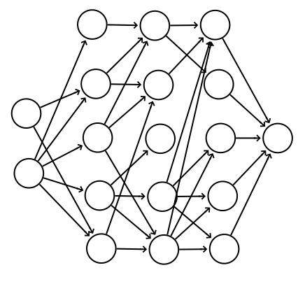
A non-intuitive regularization method called dropout discourages weights with large values. To avoid overfit, we do not want weights to be too dominating. By randomly dropping connections from one layer to the other layer, we force the network not to depend too much on a single node and try to draw prediction from many different pathways. This has an effect similar to forcing the weights smaller.

In the following diagram, for each iteration during training, we randomly drop off some connections.

Here is the code to implement the dropout for the forward feed and back propagation. In the forward feed, it takes a parameter on the percentage of nodes to be dropout. Notice that, dropout applies to training only.

def dropout_forward(x, dropout_param):
  p, mode = dropout_param['p'], dropout_param['mode']
  if 'seed' in dropout_param:
    np.random.seed(dropout_param['seed'])

  mask = None
  out = None

  if mode == 'train':
    drop = 1 - p
    mask = (np.random.rand(*x.shape) < drop) / drop
    out = x * mask
  elif mode == 'test':
    out = x

  cache = (dropout_param, mask)
  out = out.astype(x.dtype, copy=False)

  return out, cache

def dropout_backward(dout, cache):
  dropout_param, mask = cache
  mode = dropout_param['mode']
  
  if mode == 'train':
    dx = dout * mask
  elif mode == 'test':
    dx = dout
  return dx

Dropout forces the decision not to dependent on few features. It behave like other regularization in constraining the magnitude of \(W\).

Grid search for hyperparameters

Some hyperparameters are strongly related. We should tune them together with a mesh of possible combinations in a logarithmic scale. For example, for 2 hyperparameters \(\lambda\) and \(\gamma\), we start from the corresponding initial value and drop it by a factor of 10 in each step:

• (\(e^{-1}, e^{-2}, …\) and \(e^{-8}\)) and,
• (\(e^{-3}, e^{-4}, ...\) and \(e^{-6}\)).

The corresponding mesh will be \([(e^{-1}, e^{-3}), (e^{-1}, e^{-4}), \dots , (e^{-8}, e^{-5})\) and \((e^{-8}, e^{-6})]\).

Instead of using the exact cross points, we randomly shift those points slightly. This randomness may lead us to some surprises that otherwise hidden. If the optimal point lays in the border of the mesh (the blue dot), we retest it further in the boarder region.

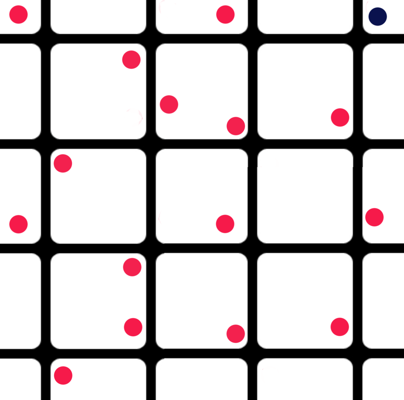
We start tuning parameters in coarse grain using fewer training iterations. In later fine tuning, we increase the iterations and drop the grid value by a factor of 3 or even smaller.

Data augmentation

One significant improvement for the DL training is to have more data. This avoids overfitting with better coverage of the feature spaces. However, getting labeled dataset can be expensive. One alternative is data augmentation. For example, for visual recognition, we can flip the image, slightly rotate or skew the images with software libraries. This helps us to avoid overfitting and produces generalized predictions invariant of the spatial transformation of the objects. Semi-learning may even expand the classification training dataset further by allowing some data without labels to be used as training data if the model can classify them with high certainty.

Very simple effort to augment your data can have a significant impact on the training.

Model ensembles

In machine learning, we can take votes from a number of decision trees to make predictions. It works because mistakes are often localized: there is a smaller chance for two models making the same mistakes. In DL, we start training with random guesses (providing random seeds are not explicitly set) and the optimized models are not unique. We pick the best models after many runs using the validation dataset. We take votes from those models to make final predictions. This method requires running multiple sessions, and can be prohibitively expensive. Alternatively, we run the training once and checkpoints multiple models. We pick the best models from the checkpoints. With ensemble models, the predictions can based on:

• one vote per model,
• weighted votes based on the confidence level of it’s prediction.

Model ensembles are very effective in pushing the accuracy up a few percentage points in some problems and very common in some DL competitions.

Reproducible Results

We initialize our model’s parameters with random values. It is hard to trouble shoot a model when output is constantly changing. It adds complexity for others to reproduce your experiments. Hence, we should set the seeds to be a known value so our result is reproducible.

import random
import numpy as np
import tensorflow as tf

random.seed(567)
np.random.seed(1234)
tf.set_random_seed(245)

However, if we use model ensembles or model averaging, we may undo the code for our final model selections so we can have different models trained from different seeds.

Convolution Net (CNN) & Long short term memory (LSTM)

FC network is rarely used alone. Exploring all possible connections among nodes in the previous layer provides a complex model that can be wasteful with small returns. A lot of information is localized. For an image, we want to extract features from neighboring pixels. CNN applies filters to explore localized features first, and then apply FC to make predictions. LSTM applies time feedback loop to extract time sequence information. This article covers the fundermental in DL that will be needed for CNN and LSTM.

Two separated articles on CNN and LSTM will explain each design in details.

Troubleshooting

Many places can go wrong when training a deep network. Here are some tips:

• Create a baseline with a simple or known network (like VGG) for data verification and comparison.
• Start with a simple network that works: fewer layers, customization and regularization layers.
• Sample and verify training data, labels in a few batches.
• Do not waste time on a large dataset with long iterations or large data batch during early development.
• Verify the trainable parameters initialization.
• Verify the range of the input and the output. (like [-1, 1] or [0, 1])
• Create simple scenarios for verification during early development:
  • Does early training beats random guessing?
  • Turn off non-critical options (e.g. regularization, data augmentation).
  • Verify if loss and accuracy improves during training.
  • Overfit with a tiny dataset. The loss should drop quickly towards 0 with regularization off.
• If loss remains high or gradient approaches NaN, experiment different learning rates.
  • For NaN, decrease the rate every time by a factor of 10.
  • If \(\Delta W\) is tiny, increase the rate every time by a factor of 10.
• Sample and visualize model’s outputs.
• Visualize the model’s parameters and activations.
  • Ideal activations should be zero centered. Add batch normalization if needed.
  • Sign of exploding gradients or diminishing gradients (too many dead nodes).
  • Ideal \(W\) and \(b\) should be normal distributed and not too high.
• Monitor gradients and \(\Delta W\) closely.
• Display and analysis samples that have wrong predictions.
• Start your tuning from overfit first (with less regularization).
• The dataset should have similar amount of datapoints in each class.
• When adding regularization, tune the regularization factor properly.

Design consideration:

• Always keep track of the shape of the data and document it in the code.
• Rescale your input features in particular for non-imaging data.
• Initialize all random seeds to produce repeatable results.
• Use academic dataset first if possible.
• Verify the quality of any custom dataset.
  • Choose related categories addressing your target problem.
  • Filter out low quality samples.
• Start with standard loss functions before any customization.
• Record output periodically for verification.
• Version control models and save model checkpoints for different hyperparameters for easy reproduction.
• Add data shuffling after early development.
• If NaN happens and gradient is too high, apply gradient clipping. (in particular for RNN)

If you need to implement custom layers:

• Unit test the forward pass and back propagation code.
• At the beginning, test with non-random data.
• Compare the backpropagation result with the naive gradient check.
• Add tiny \(\epsilon\) for divison or log computation to avoid NaN.

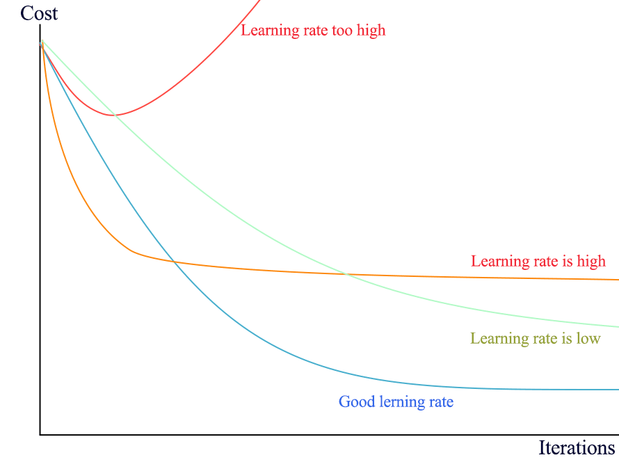
Monitor loss

We want to plot the cost vs iterations. Monitor the loss to see its trend:

• If loss goes up early, the learning rate is way too high.
• If loss drops fast and flattens very quickly, the learning rate is high.
• If loss drops too slow, the learning rate is too slow.

If the learning rate is too large, we may also see a sudden jump in loss:

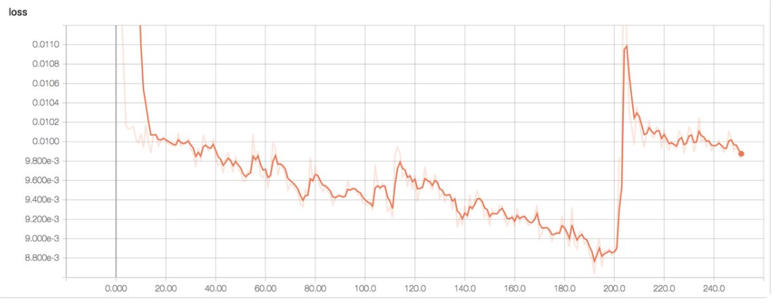
(Image source Emil Wallner)

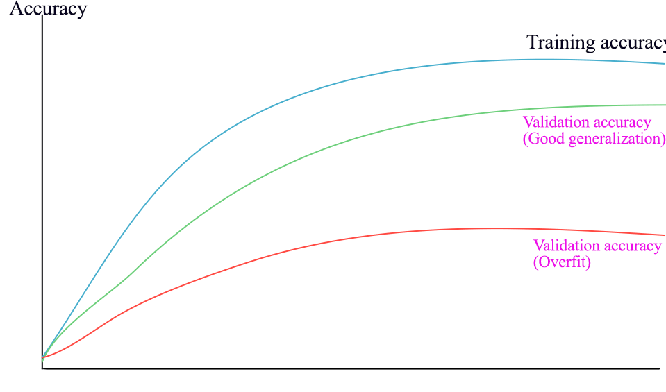
Train vs validation accuracy

Plot out accuracy between validation and training to identify overfit issues.

• If validation error is much lower than the training error, the model is overfit.

Monitor Gradient descent

Monitor the updates to \(W\) ratio:

• If the ratio is \(> 1e-3\), consider lower the learning rate.
• If the ratio is \(< 1e-3\), consider increase the learning rate.

Plot weight, activation and gradient histograms for all layers.

• Verify if you are having gradient diminishing or explode problem.
• Identify layers that have very low gradients.
• Verify whether you have too many saturated nodes.

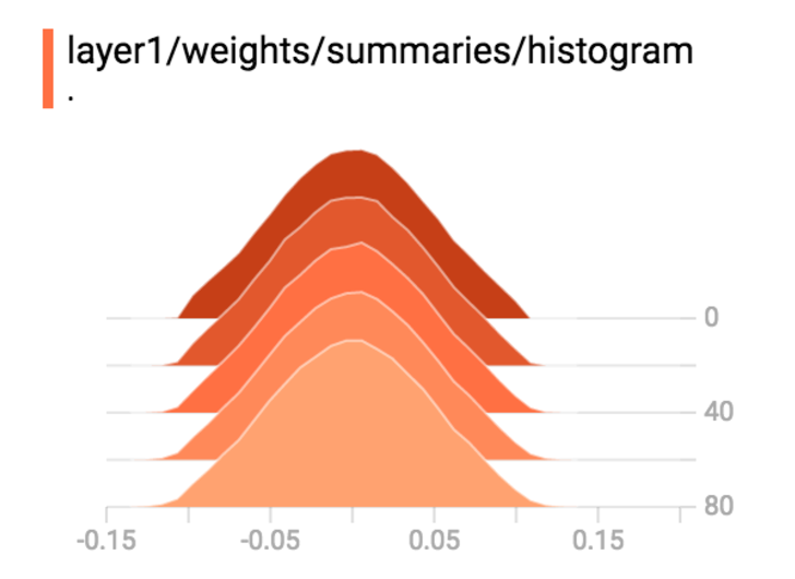
Here is the gradient plot for a variable. It will be un-healthy if

• All close to 0. (gradient is diminishing)
• Too large positively or negatively. (gradient is exploding)
• All positive or all negative. (the gradient descent is zip-zapping)

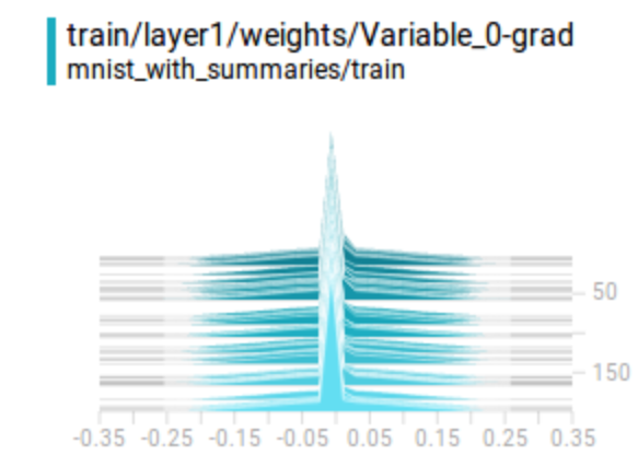
Here is the code in creating gradient summary:

with tf.name_scope('train'):
    optimizer = tf.train.AdamOptimizer()
    # Get the gradient pairs (Tensor, Variable)
    grads = optimizer.compute_gradients(cross_entropy)
    # Update the weights wrt to the gradient
    train_step = optimizer.apply_gradients(grads)
    # Save the grads with tf.summary.histogram
    for index, grad in enumerate(grads):
        tf.summary.histogram("{}-grad".format(grads[index][1].name), grads[index])

(Source LH Franc)

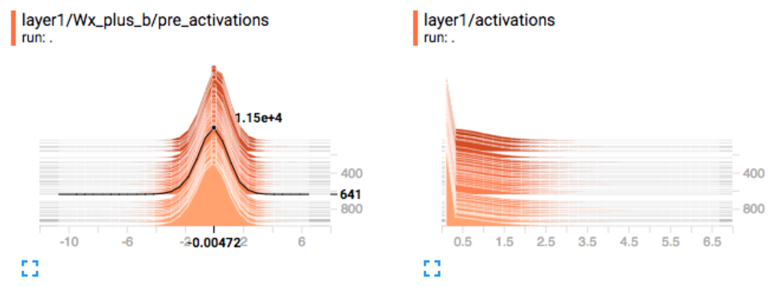
Activation

For gradient descent to perform the best, the nodes’ outputs before the activation function should be normal distributed. For example, we should apply a batch normalization to correct the non-zero centered pre-activation output below. The right side plot is the activation output of a ReLU function. It will be bad if there are too many dead or highly activated nodes.

Visualize filters and activation

For visualization problem, we can visualize the \(W\) matrix in 2D for FC network, or the filters for CNN in the first couple layers. This helps us to identify what type of features that the model is extracting. The first layer should extract simple structures like edge and color.

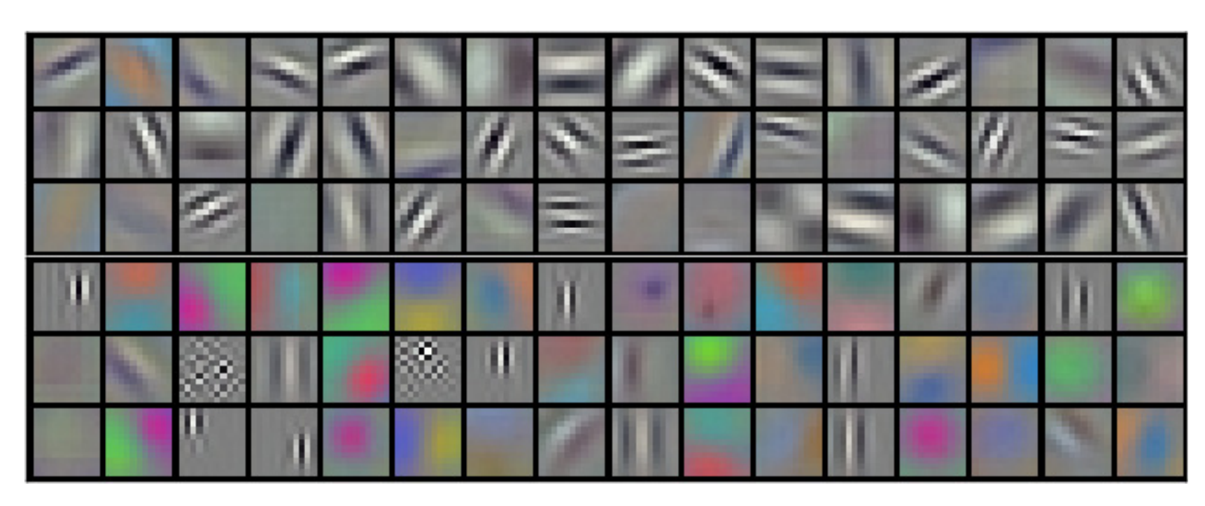
We can locate pictures that have the highest activation for each feature map. Once again, it verifies what features are used in building the model.

In later layers, we should see more complex structures evolved:

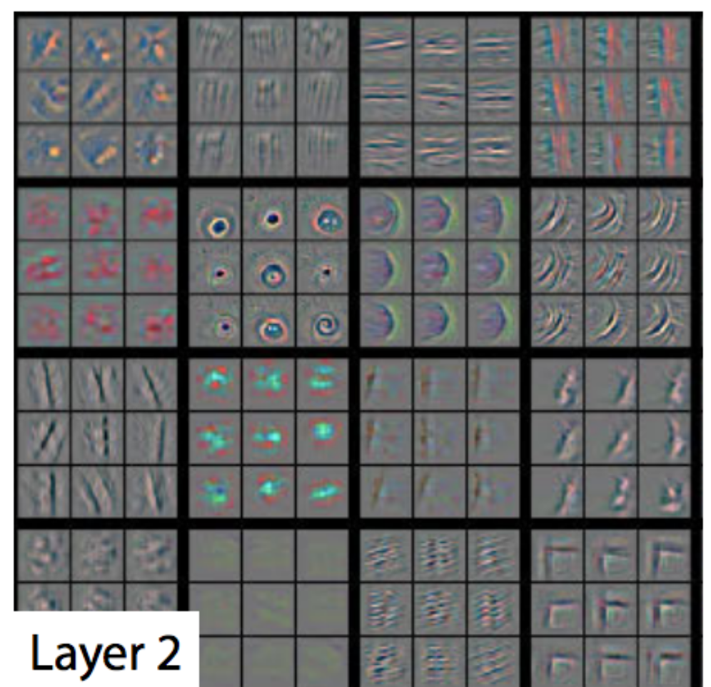
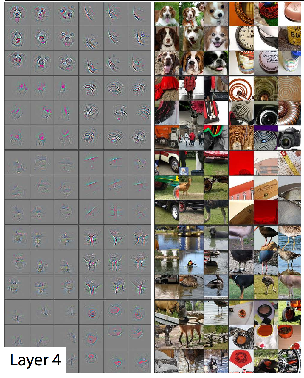
(Source from Visualizing and Understanding Convolutional Networks, Matthew D Zeiler et al.)

Maximum likelihood estimation (MLE)

We state without proof that KL divergence and cross entropy is a good cost function. This is actually not a random guess. Let’s derive it.

What is our objective in training a model? We want to find \(W\) such that our training dataset is most possible comparing to other \(W\) (Maximum likelihood estimation MLE).

The probability of the observed training datapoints based on our model is:

for training datapoints \(x_i\) with corresponding true label \(y_i\).

The optimal model parameters \(W^{*}\) in MLE is simply:

Negative log-likelihood (NLL)

Logarithm is a monotonic function. Hence optimize \(J\) is the same as optimize \(\log{J}\). However, \(\log{(probability)}\) changes the sign. Therefore Maximum likelihood is translated to minimize the negative log-likelihood NLL. As shown below, NNL is preferable over MLE because it involves additions (easier and more stable) but not multiplications.

Maximize the MLE is the same as minimizing NNL.

NNL is mathematically the same as cross entropy.

Lost function for logistic classifier

NNL is very powerful. It provides a formal way to derive a cost function. To illustrate that, we apply NNL to a logistic classifier to find its cost function.

The probability for the output \(y_i\) is defined by the logistic function \(\sigma\) as:

Apply NLL,

The total sum becomes

This is indeed called the logistic loss which we use for the logistic classifier.

Summary

Let’s have a brief summary:

• MLE find the best model’s parameters for the observed data.
• Optimizing MLE is the same as optimizing NNL but NNL is easier.
• NNL and cross entropy are mathematically the same.
• Optimize cross entropy is the same as optimize KL-divergence.
• NNL is good for derving a cost function.

Credits

For the CIFRA 10 example, we start with assignment 2 in the Stanford class “CS231n Convolutional Neural Networks for Visual Recognition”. We start with some skeleton codes provided by the assignment and put it into our code to complete the assignment.