“Deep learning without going down the rabbit holes.”
What is deep learning (DL)?
Deep learning is about building a function estimator. Historically, people explain deep learning (DL) using the neural network. Nevertheless, deep learning has outgrown this explanation.
Let’s build a new android named Pieter. Our first task is to teach Pieter to recognize objects. Can the human visual system be replaced by a big function estimator?
Deep learning has many scary looking equations. We will walk through examples to show how it works. Most of them are pretty simple.
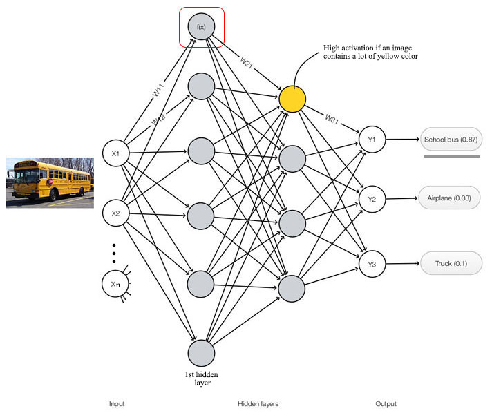
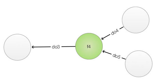
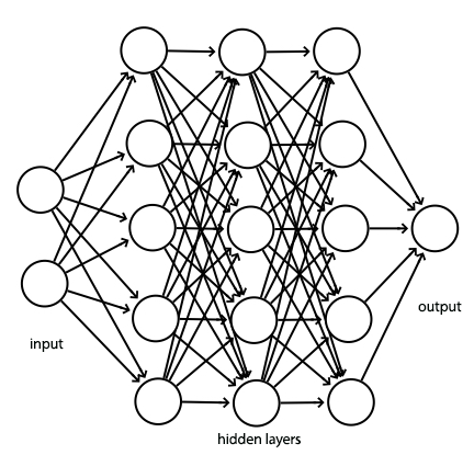
A deep network composes of layers of nodes. Our network above has one input layers, two hidden layers and one output layer. We compute the output of each node with:
\[z_j = \sum_{i} W_{ij} x_{i} + b_{j}\]where \(x_{i}\) are the output from the previous layer, \(W_{ij}\) are the weights between node \(i\) and \(j\), and \(b_j\) is the bias. Finally, the node convert \(z_j\) to a value between 0 and 1 using a sigmoid function.
\[f(z_j) = \frac{1}{1 + e^{-z_j}}\]For example, we have a grayscale image with just four pixels (0.1, 0.3, 0.2, 0.1). We assume the weights \(W\) and the bias \(b\) are (0.3, 0.2, 0.4, 0.3) and -0.8 respectively. The output of the node is:
\[\begin{split} z_j & = 0.3 \cdot 0.1 + 0.2\cdot 0.3 + 0.4\cdot0.2 + 0.3\cdot0.1 - 0.8 = -0.6 \\ f(z_j) &= \frac{1}{1 + e^{0.6}} = 0.35 \end{split}\]In this network, we make 3 predictions. \(Y_1\) is the probability that the image is a school bus. The other two outputs represent the probability of two other object classes.
\(x_{i}\) is called the feature in DL. A deep network extracts features in the training data to make predictions. For example, one of the nodes may be trained to detect the yellow color. For a yellow school bus, the activation of that node should be high. The essence of DL is to learn \(W\) and \(b\) from the training data (training dataset). In this exercise, we supply all the weight and bias values to our android Pieter. But as the term “deep learning” implies, Pieter will learn those parameters by himself using the training dataset. We still miss a few pieces for the puzzle, but the deep network diagram and the equations above are the major foundation for the deep learning.
XOR
Can a DL network model a logical function? For the skeptics, we will build an “exclusive or” (a xor b) function using a simple network with \(W\) and \(b\) shown as below:
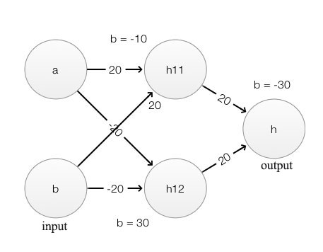
For each node, we apply the same equations mentioned previously:
\[z_j = \sum_{i} W_{ij} x_i + b_{j}\] \[h_j = \sigma(z) = \frac{1}{1 + e^{-z_j}}\]Let’s use a Python scientific package called numpy to compute the output of our network.
We provide coding to help the audience to understand the mechanism in details. Nevertheless, a full understanding of this code is not required.
import numpy as np

def sigmoid(x):
  return 1 / (1 + np.exp(-x))

def layer1(x1, x2):
    w11, w21, b1 = 20, 20, -10
    w12, w22, b2 = -20, -20, 30

    v = w11*x1 + w21*x2 + b1
    h11 = sigmoid(v)

    v = w12*x1 + w22*x2 + b2
    h12 = sigmoid(v)

    return h11, h12

def layer2(x1, x2):
    w1, w2, bias = 20, 20, -30

    v = w1*x1 + w2*x2 + bias
    return sigmoid(v)

def xor(a, b):
    h11, h12 = layer1(a, b)
    return layer2(h11, h12)          # Feed the output of last layer to the next layer

print(" 0 ^ 0 = %.2f" % xor(0, 0))   # 0.00
print(" 0 ^ 1 = %.2f" % xor(0, 1))   # 1.00
print(" 1 ^ 0 = %.2f" % xor(1, 0))   # 1.00
print(" 1 ^ 1 = %.2f" % xor(1, 1))   # 0.00
As the output of our code show, this network provides the XOR function as expected:
 0 ^ 0 = 0.00
 0 ^ 1 = 1.00
 1 ^ 0 = 1.00
 1 ^ 1 = 0.00
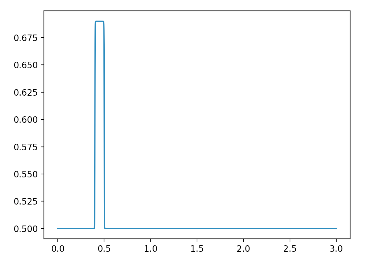
Delta function
Back to basic calculus, a function can be constructed with infinite narrow rectangles (a.k.a. delta function). If we can construct a delta function using a network, we can combine them for any functions.
Here is the code using the same equations and network layout, but with different parameters:
import numpy as np
import matplotlib.pyplot as plt

def sigmoid(x):
  return 1 / (1 + np.exp(-x))

def layer1(x):
    h11 = sigmoid(1000 * x - 400)
    h12 = sigmoid(1000 * x - 500)
    return h11, h12

def layer2(v1, v2):
    return sigmoid(0.8 * v1 - 0.8 * v2)

def func_estimator(x):
    h11, h12 = layer1(x)
    return layer2(h11, h12)

x = np.arange(0, 3, 0.001)
y = func_estimator(x)

plt.plot(x, y)
plt.show()
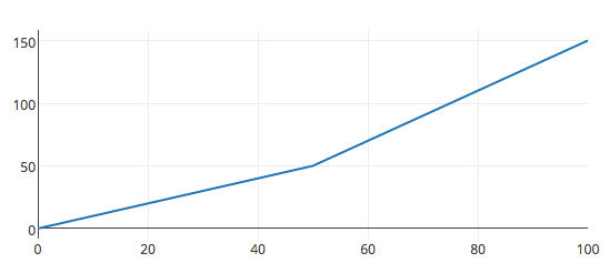
As shown below, this network produces a delta like function when we plot its output.
Implementing an XOR or a delta function is not important for DL. Nevertheless, we demonstrate the possibilities of building a complex function estimator through a network of simple computation nodes. A three-layer network can recognize hand written numbers with an accuracy of 95+%. The deeper a network; the more powerful it is. For example, Microsoft ResNet for visual recognition contains 151 layers with million trainable parameters. For many problems, the real models behind them are very complex. In autonomous driving, we can model a policy (turn, accelerate, or brake) to imitate what human do based on what they see. This policy is too difficult to model analytically. Alternatively, a deep learning network can be trained well enough to make similar actions as real drivers.
If we cannot solve a problem analytically, then train a model empirically.
Build a Linear Regression Model
Deep learning acquires its knowledge from training data. Pieter learns the model parameters \(W\) by processing training data. For another example, Pieter wants to expand his horizon and start online dating. He wants to know how many dates he will get according to his years of education and monthly income. Let’s model it with a simple linear equation:
\[dates = W_1\times \text{years in school} + W_2 \times \text{monthly income} + b\]He surveys 1000 people on their income, education and their number of online dates. The number of dates (answers) in the training dataset are called the true values or true labels. The task for Pieter is to find the parameters \(W\) and \(b\) using the training data collected by the survey.
The steps are:
- Take a first guess on W and b.
- Use the model to compute the result for each sample in the training dataset.
- Find the average error between the computed values and the true values.
- Compute how fast the error may increase or drop relative to W and b. (Gradient descent)
- Re-adjust W & b accordingly to reduce the average error.
We repeat step 2 to 5 many times until \(W\) and \(b\) until the average error is very small for our samples.
Gradient descent
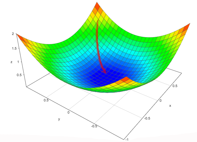
Deep learning is about learning how much it costs. Step 4 and 5 is called the gradient descent in DL. We need a function to measure how good our model is. In DL, it is called the cost function or loss function. It measures the difference between our model and the real world. Mean square error (MSE) between the true labels and the predicted values is one obvious candidate.
\[MSE= J(\hat{y}, y, W, b) = \frac{1}{N} \sum_i (\hat{y}_i - y_i)^2\]where \(\hat{y}_i\) is the model prediction and \(y_i\) is the true value for sample \(i\). We add all the sample errors and take the average. We can visualize the cost below with x-axis being \(W_1\), y-axis being \(W_2\) and z-axis being the average cost \(J\). To find our model, we need to find the optimal values for \(W_1\) and \(W_2\) with the lowest cost. In short, what are the model parameters with the lowest error for our samples.The mechanism to find the lowest cost is similar to dropping a marble at a random point \((W_1, W_2)\) and let gravity do its work.
There are different cost functions with different objectives and solutions. Some functions are easier to optimize and some may be less sensitive to outliers. Nevertheless, finding a cost function is one critical factor in building a DL.
Optimizing \(W\) means finding the trainable parameters with lowest cost.
Learning rate
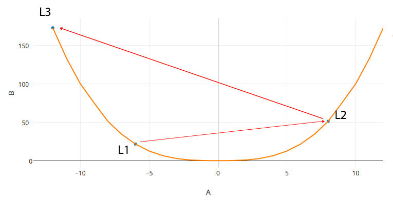
Thinking in 3 dimension is hard.
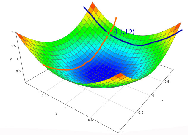
Let’s simplify it in 2-D first. Consider a point at (L1, L2) where we cut through the diagram along the blue and orange line, then we plot those curves in a 2D diagram.
The x-axis is \(W\) and the y-axis is the cost.
Train a model with gradients: To lower cost, we move \(L_1\) to the right to find the lowest cost. But by how much? L2 has a smaller gradient than L1. i.e. the cost drop faster alone \(W_1\) direction than \(W_2\). Like dropping a ball at (L1, L2), we expect the ball drops faster in the \(W_1\) direction. Therefore, the adjustment for \((W_1, W_2)\) should be proportional to its partial gradient at that point. i.e.
\[\Delta W_i \propto \frac{\partial J}{\partial W_i}\] \[\text{ i.e. } \Delta W_1 \propto \frac{\partial J}{\partial W_1} \text{ and } \Delta W_2 \propto \frac{\partial J}{\partial W_2}\]Add a ratio value \(\alpha\), the adjustments to \(W\) becomes:
\[\Delta W_i = \alpha \frac{\partial J}{\partial W_i}\] \[W_i = W_i - \Delta W_i\]At L1, the gradient is negative and therefore we are moving \(W_1\) to the right. The variable \(\alpha\) is called the learning rate. A small learning rate learns slowly: a small learning rate changes \(W\) slowly and takes more iterations to locate the minimum. However, the gradient is less accurate when we use a larger step. In DL, finding the right value for the learning rate is a trial and error exercise which depends on the problem you are solving. We usually try values ranging from \(1e^{-7}\) to 1 in logarithmic scale (\(1e^{-7}, 1e^{-6}, 1e^{-5}, \dots, 1)\). Parameters such as the learning rate are called hyperparameters because they need to be tunned.
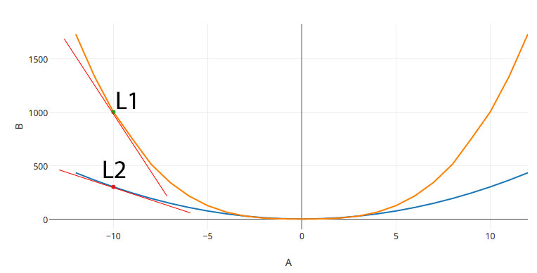
A large learning rate can have serious problems. It costs \(w\) to oscillate with increasing cost:
Let’s start with w = -6 (L1). If the gradient is huge and the learning rate is large, \(w\) will swing too far to the right (L2) that may even have a larger gradient. Eventually, rather than dropping down slowly to a minimum, \(w\) oscillates upward to a higher cost.
A large learning rate overshoots your target. Here is an illustration on some real life problems like natural language processing (NLP). When we gradually descend on a slope, we may land in an area with a steep gradient in which bounces \(W\) all the way back. It is very difficult to find the minimum with a constant learning rate with this kind of cost function shape. Advanced methods to address this problem will be discussed later.
Naive gradient checking
There are many ways to compute a partial derivative. One naive but important method is using the simple partial derivative definition.
\[\frac{\partial f}{\partial x} = \frac{f(x+\Delta x_i) - f(x-\Delta x_i) } { 2 \Delta x_{i}}\]Here is a simple code demonstrating the derivative of \(x^2 \text{ at } x = 4\)
def gradient_check(f, x, h=0.00001):
  grad = (f(x+h) - f(x-h)) / (2*h)
  return grad

f = lambda x: x**2
print(gradient_check(f, 4))
We never use this method in production; however, computing partial derivative is tedious and error prone. We often use the naive method to verify a partial derivative implementation during development.
Mini-batch gradient descent
When computing the cost function, we add all the errors for the entire training dataset. This takes too much time for just one round of parameter update. On the contrary, we can perform stochastic gradient descent which makes one \(W\) update per training sample. Nevertheless, the gradient descent will follow a zip zap pattern rather than the curve of the cost function. When it gets close to the minimum, it may continuously zip zag around the minimum region.
A good compromise is to process a batch of N samples at a time. The batch size N is a tunable hyperparameter, but usually not very critical. We can start with 64 samples for lower memory consumptions.
\[J = \frac{1}{N} \sum_i (\hat{y}_i - y_i)^2\]Backpropagation
Backpropagate your loss to adjust W. To compute the partial derivatives, \(\frac{\partial J}{\partial W_i}\), we can start from each node in the left most layer and calculate the gradient until it reaches the rightmost layer. Then, we move to the next layer and start the process again. For a deep network, this is very inefficient. To compute the partial gradient efficiently, we perform a forward pass and compute the gradient by a single backpropagation.
Forward pass
The method forward computes the output:
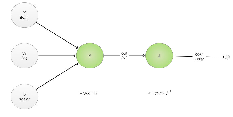
\[out = W_1 X_1 + W_2 X_{2} + b\]def forward(x, W, b):
# x: input sample (N, 2)
# W: Weight (2,)
# b: bias float
# out: (N,)
out = x.dot(W) + b # X * W + b: (N, 2) * (2,) -> (N,)
return out
To compute the mean square loss:
\[J = \frac{1}{N} \sum_i (out - y_{i})^2\]def mean_square_loss(out, y):
# h: prediction (N,)
# y: true value (N,)
N = X.shape[0] # Find the number of samples
loss = np.sum(np.square(out - y)) / N # Compute the mean square error from its true value y
return loss
Backpropagation pass
Find the derivative by backpropagation. We backpropagate the gradient from the right most layer to the left in one single pass. In the programming code, we often name our backpropagation derivative as:
\[\frac{\partial J}{\partial out} \text{ as dout}\] \[\frac{\partial out}{\partial var} \text{ as dvar}\]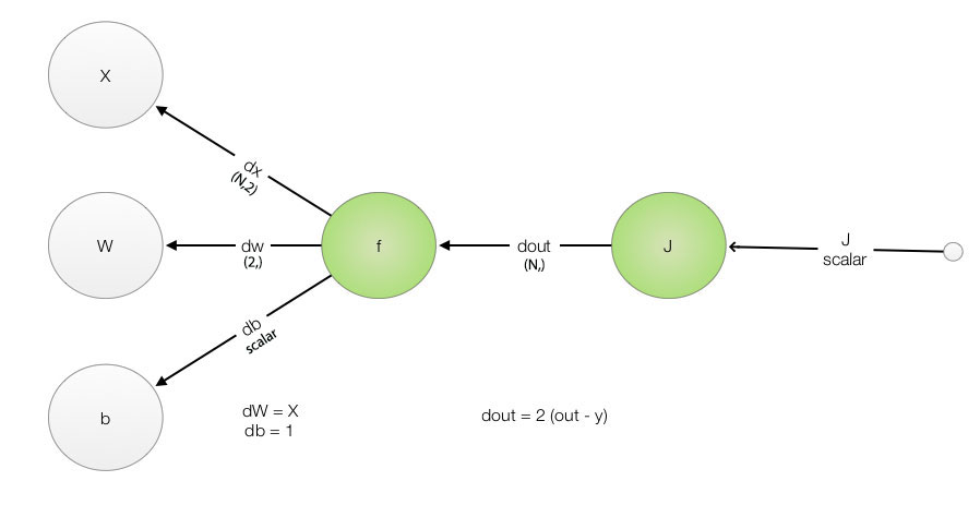
Keep track of the naming of your input and output as well as its shape (dimension). This is one great tip when you program DL. (N,) means a 1-D array with N elements. (N,1) means a 2-D array with N rows each containing 1 element. (N, 3, 4) means a 3-D array.
First, compute the first partial derivative \(\frac{\partial J}{\partial out_i}\) in the right most layer.
\[J = \frac{1}{N} \sum_i (out_i - y_i)^2\] \[J_i = \frac{1}{N} (out_i - y_i)^2\] \[\frac{\partial f}{\partial out_i} = \frac{2}{N} (out_i - y_i)\]We add a line of code in the mean square loss to compute \(\frac{\partial J}{\partial out_{i}}\)
def mean_square_loss(h, y):
    # h: prediction (N,)
    # y: true value (N,)
    ...
    dout = 2 * (h-y) / N      # Compute the partial derivative of J relative to out
    return loss, dout
Use the chain rule to backpropagate the gradient. Now we have \(\frac{\partial J}{\partial out_i}\) . We apply the simple chain rule in calculus to backpropagate the gradient one more layer to the left.
\[\frac{\partial J}{\partial W} = \frac{\partial J}{\partial out} \frac{\partial out}{\partial W}\] \[\frac{\partial J}{\partial b} = \frac{\partial J}{\partial out} \frac{\partial out}{\partial b}\]We follow our naming convention to name \(\frac{\partial J}{\partial W} \text{ as dW}\) and \(\frac{\partial J}{\partial b} \text{ as db}\).
With output as:
\[out = W X + b\]The partial derivatives are:
\[\frac{\partial out}{\partial W} = X\] \[\frac{\partial out}{\partial b} = 1\]Apply the derivative to the chain rule:
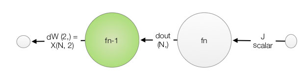
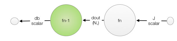
\[\frac{\partial J}{\partial W} = \frac{\partial J}{\partial out} \frac{\partial out}{\partial W} = \frac{\partial J}{\partial out} X\] \[\frac{\partial J}{\partial b} = \frac{\partial J}{\partial out} \frac{\partial out}{\partial b} = \frac{\partial J}{\partial out}\]A lot of mathematical notation is involved, but the code for \(dW, db\) is pretty simple.
def forward(x, W, b):
    out = x.dot(W) + b
    cache = (x, W, b)
    return out, cache

def backward(dout, cache):
    # dout: dJ/dout (N,)
    # x: input sample (N, 2)
    # W: Weight (2,)
    # b: bias float
    x, W, b = cache
    dW = x.T.dot(dout)            # Transpose x (N, 2) -> (2, N) and multiple with dout. (2, N) * (N, ) -> (2,)
    db = np.sum(dout, axis=0)     # Add all dout (N,) -> scalar
    return dW, db

def compute_loss(X, W, b, y=None):
    h, cache = forward(X, W, b)

    loss, dout = mean_square_loss(h, y)
    dW, db = backward(dout, cache)
    return loss, dW, db
Here is the full listing of the code for your quick reference:
import numpy as np

iteration = 10000
learning_rate = 1e-6
N = 100

def true_y(education, income):
    """ Find the number of dates corresponding to the years of education and monthly income.
    Instead of collecting the real data, an Oracle provides us a formula to compute the true value.
    """
    dates = 0.8 * education + 0.003 * income + 2
    return dates

def sample(education, income):
    """We generate sample of possible dates from education and income value.
    Instead of collecting the real data, we find the value from the true_y
    and add some noise to make it looks like sample data.
    """
    dates = true_y(education, income)
    dates += dates * 0.01 * np.random.randn(education.shape[0]) # Add some noise
    return dates

def forward(x, W, b):
    # x: input sample (N, 2)
    # W: Weight (2,)
    # b: bias float
    # out: (N,)
    out = x.dot(W) + b        # Multiple X with W + b: (N, 2) * (2,) -> (N,)
    cache = (x, W, b)
    return out, cache

def mean_square_loss(h, y):
    # h: prediction (N,)
    # y: true value (N,)
    N = X.shape[0]            # Find the number of samples
    loss = np.sum(np.square(h - y)) / N   # Compute the mean square error from its true value y
    dout = 2 * (h-y) / N                  # Compute the partial derivative of J relative to out
    return loss, dout

def backward(dout, cache):
    # dout: dJ/dout (N,)
    # x: input sample (N, 2)
    # W: Weight (2,)
    # b: bias float
    x, W, b = cache
    dw = x.T.dot(dout)            # Transpose x (N, 2) -> (2, N) and multiple with dout. (2, N) * (N, ) -> (2,)
    db = np.sum(dout, axis=0)     # Add all dout (N,) -> scalar
    return dw, db

def compute_loss(X, W, b, y=None):
    h, cache = forward(X, W, b)

    if y is None:
        return h

    loss, dout = mean_square_loss(h, y)
    dW, db = backward(dout, cache)
    return loss, dW, db


education = np.random.randint(26, size=N) # (N,) Generate 10 random sample with years of education from 0 to 25.
income = np.random.randint(10000, size=education.shape[0]) # (N,) Generate the corresponding income.

# The number of dates according to the formula of an Oracle.
# In practice, the value come with each sample data.
Y = sample(education, income)    # (N,)
W = np.array([0.1, 0.1])         # (2,)
b = 0

X = np.concatenate((education[:, np.newaxis], income[:, np.newaxis]), axis=1) # (N, 2) N samples with 2 features

for i in range(iteration):
    loss, dW, db = compute_loss(X, W, b, Y)
    W -= learning_rate * dW
    b -= learning_rate * db
    if i%100==0:
        print(f"iteration {i}: loss={loss:.4} W1={W[0]:.4} dW1={dW[0]:.4} W2={W[1]:.4} dW2={dW[1]:.4} b= {b:.4} db = {db:.4}")

print(f"W = {W}")
print(f"b = {b}")
General principle in backpropagation
With vectorization and some ad hoc functions, backpropagation can be error prone, but not necessarily difficult. Let’s summarize the steps above with some good tips.
Draw the forward pass and backpropagation pass with all variable names. Add functions, derivatives and the shape for easy reference.
Perform a forward pass to calculate the output and the cost:
\[out = W_1 X_{1} + W_2 X_{2} + b\] \[J = \frac{1}{N} \sum_i (out - y_{i})^2\]Find the partial derivative of the cost:
\[\frac{\partial J}{\partial out} = \frac{2}{N} (out - y)\]For every node, find the derivative of the function:
\[out = W X + b\] \[\frac{\partial out}{\partial W} = X\] \[\frac{\partial out}{\partial b} = 1\]Find the gradient by applying the chain rule from right to left:
\[\frac{\partial J}{\partial l_{k-1}} = \frac{\partial J}{\partial l_{k}} \frac{\partial l_k}{\partial l_{k-1}}\]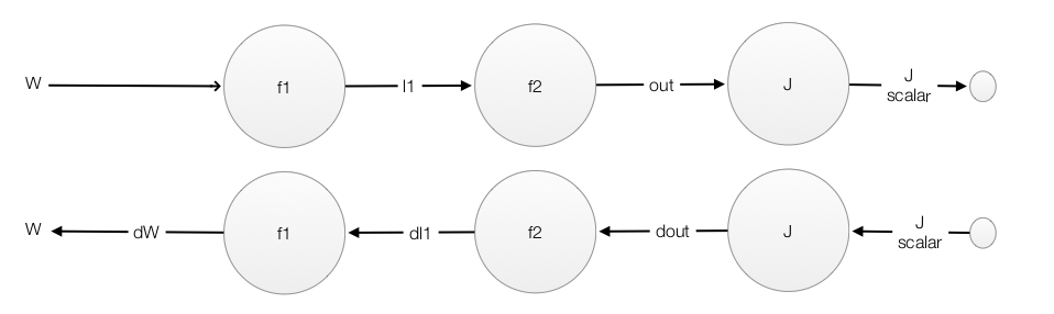
Similary,
\[\text{dW} = \text{dl1} \frac{\partial f_{1}}{\partial W}\]Know the shape (dimension) of your variables. Always make the shape (dimension) of the variables clear in the diagram and in the code. Use this information to verify your math operations. For example, multiplying a (N, C, D) matrix with a (D, K) matrix should produce a (N, C, K) matrix. Vectorization may confuse you. Expand the equation with sub-indexes with only a couple of weights and features so you can work through the math.
Many deep learning software platforms provide pre-built layers with feed forward and backpropagation.
More on backpropagation
In backpropagation, we may back propagate multiple paths back to the same node. To compute the gradient correctly, we need to add both paths together:
Testing the model
I strongly recommend you to implement a linear regression model that interests you. By working with a simple model, you can create scenarios to test your theories and develop a better insight in DL. A real model is often too hard to trouble shoot to develop such insight.
So, let Pieter train the system.
iteration 0: loss=2.825e+05 W1=0.09882 dW1=1.183e+04 W2=-0.4929 dW2=5.929e+06 b= -8.915e-05 db = 891.5
iteration 200: loss=3.899e+292 W1=-3.741e+140 dW1=4.458e+147 W2=-1.849e+143 dW2=2.203e+150 b= -2.8e+139 db = 3.337e+146
iteration 400: loss=inf W1=-1.39e+284 dW1=1.656e+291 W2=-6.869e+286 dW2=8.184e+293 b= -1.04e+283 db = 1.24e+290
iteration 600: loss=nan W1=nan dW1=nan W2=nan dW2=nan b= nan db = nan
The application overflows within 600 iterations! (nan: not a number) Since the loss and the gradient above are so high, we tune the learning rate to a smaller value \(1e^{-8}\). The overflow problem is gone, but the loss remains high.
iteration 90000: loss=4.3e+01 W1= 0.23 dW1=-1.3e+02 W2=0.0044 dW2= 0.25 b= 0.0045 db = -4.633
W = [ 0.2437896   0.00434705]
b = 0.004981262980767952
With 10,000,000 iterations and even a smaller learning rate \(1e^{-10}\), the loss remains very high. It will be better to trace the source of problem now.
iteration 9990000: loss=3.7e+01 W1= 0.22 dW1=-1.1e+02 W2=0.0043 dW2= 0.19 b= 0.0049 db = -4.593
W = [ 0.22137005  0.00429005]
b = 0.004940551119084607
Tracing gradient is a powerful tool in DL debugging.
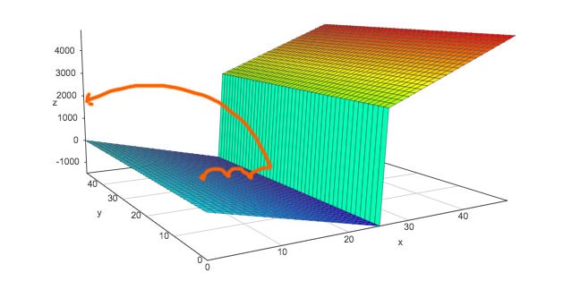
Let’s plot the cost function relative to \(W\) to illustrate the real issue.
This is a U shape curve that is different from a bowl shape curve that we used in the gradient descent explanation.
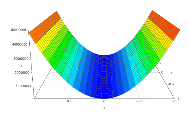

Monthly income ranges from 0 to 10,000 and years of education range from 0 to 30. The cost gradient relative to the income is much smaller than the education at the current scale. We cannot have a single learning rate that works well for both of them. We can tune a learning rate for \(W_2\) so we can learn the weight for the income at a resonable speed. But since \(W_1\) has a much bigger gradient, the jump for \(W_1\) is huge at this learning rate.
The solution is pretty simple. We re-scale the income value into a new range from 0 to 10. Income unit is now in 1K.
def true_y(education, income):
    dates = 0.8 * education + 0.3 * income + 2
    return dates

...

income = np.random.randint(10, size=education.shape[0]) # (N,) Generate the corresponding income.
This is the output for our new training:
iteration 0: loss=518.7 W1=0.1624 dW1=-624.5 W2=0.3585 dW2=-2.585e+03 b= 0.004237 db = -42.37
iteration 10000: loss=0.4414 W1=0.8392 dW1=0.0129 W2=0.3128 dW2=0.004501 b= 0.5781 db = -0.4719
iteration 20000: loss=0.2764 W1=0.8281 dW1=0.009391 W2=0.3089 dW2=0.003277 b= 0.9825 db = -0.3436
iteration 30000: loss=0.1889 W1=0.8201 dW1=0.006837 W2=0.3061 dW2=0.002386 b= 1.277 db = -0.2501
iteration 40000: loss=0.1425 W1=0.8142 dW1=0.004978 W2=0.3041 dW2=0.001737 b= 1.491 db = -0.1821
iteration 50000: loss=0.1179 W1=0.81 dW1=0.003624 W2=0.3026 dW2=0.001265 b= 1.647 db = -0.1326
iteration 60000: loss=0.1049 W1=0.8069 dW1=0.002639 W2=0.3015 dW2=0.0009208 b= 1.761 db = -0.09653
iteration 70000: loss=0.09801 W1=0.8046 dW1=0.001921 W2=0.3007 dW2=0.0006704 b= 1.844 db = -0.07028
iteration 80000: loss=0.09435 W1=0.803 dW1=0.001399 W2=0.3001 dW2=0.0004881 b= 1.904 db = -0.05117
iteration 90000: loss=0.09241 W1=0.8018 dW1=0.001018 W2=0.2997 dW2=0.0003553 b= 1.948 db = -0.03725
W = [ 0.80088848  0.29941657]
b = 1.9795590414763997
The trained model after 90K iterations is
\[dates = 0.8 \text{ education } + 0.3 \text{ (income in 1k) } + 1.98\]which is close to the true world
\[dates = 0.8 \text{ education } + 0.3 \text { (income in 1k) } + 2\]Non-linearity
Pieter comes back and complains our linear model is not adequate. Pieter claims the relationship between the years of education and the number of dates are not exactly linear. We should give more rewards for people holding advance degrees.
Can we combine 2 linear functions with multiple layers to form a non-linear function?
\[f(x) = Wx + b\] \[g(z) = Uz + c\]The answer is no.
\[g(f(x)) = U(Wx+b) + c = Vx + d\]After some thought, we apply the following to the output of a computation node.
\[f(x) = max(0, x)\]With this function, in theory, we can construct the non-linear relations that Pieter wants.
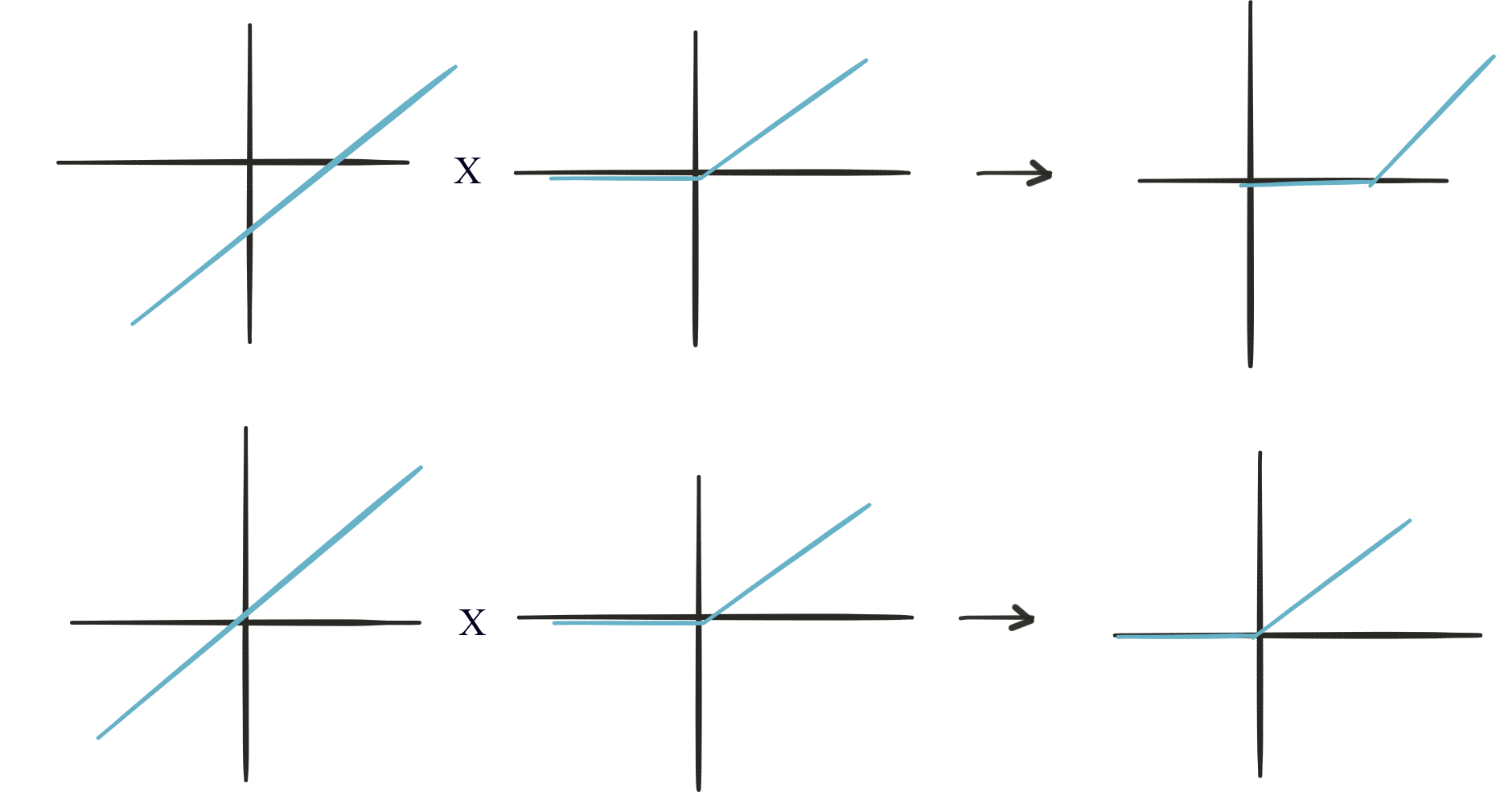
Adding both output:
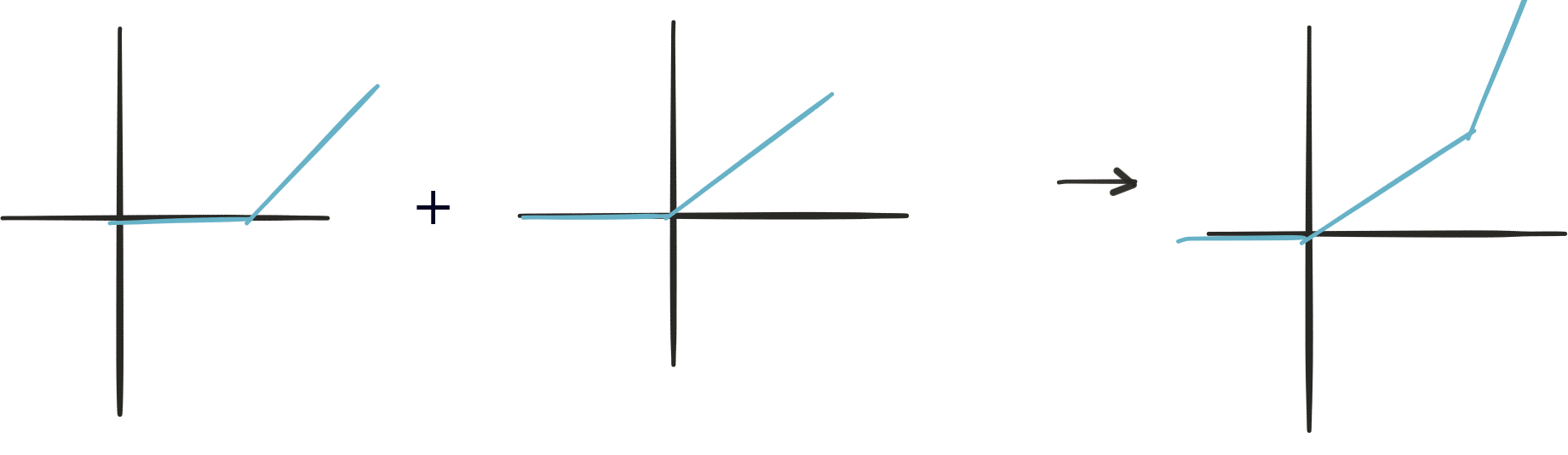
Adding a non-linear function after a linear equation enriches the complexity of our model. These methods are called activation functions. Common functions are tanh and ReLU.
Sigmoid function
Sigmoid function is one of the earliest functions used in deep networks.
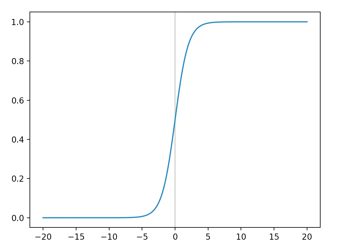
The far left and right region is flat. These areas are where neuron (node) is saturated: any change in input results in tiny change in the output. The gradient is near zero. Since backpropagation depends on the magnitude of the gradient, we learn very slow if the gradient is very small (\(\Delta W \propto gradient\)). Therefore sigmoid function is no longer used as an activation function. Instead, sigmoid function is used as the final output layer for a binary classifier (a classifier that has only one node in the output layer.)
ReLU
ReLU is one of the most popular activation functions.
\[y = max(0, x)\]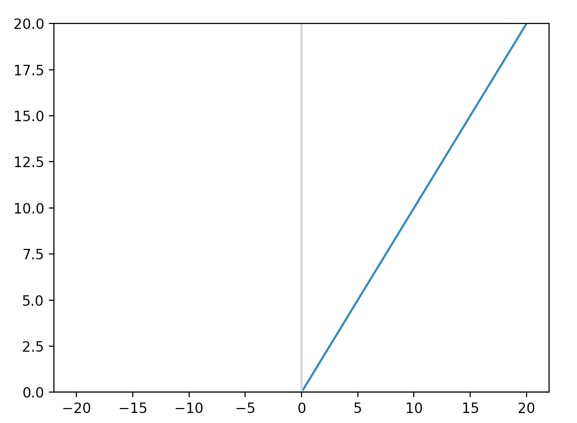
It converges faster to the optimized solution because it is less easy to be saturated comparing with sigmoid or tanh. Also computing ReLU is simple without expensive exponential function.
ReLU is most common comparing with other activation functions
Leaky ReLU
However, ReLU may have some disadvantage. A ReLU node can die, but even worst stays dead in the flat saturated region. A dead node keep data from feeding forward and stop training \(W\) backward in the backpropagation. Some deep network with ReLU has large amount of dead nodes if the learning rate is set too high. Leaky ReLU addresses the problem by having a slightly slopped line instead of a flat region when \(x < 0\).
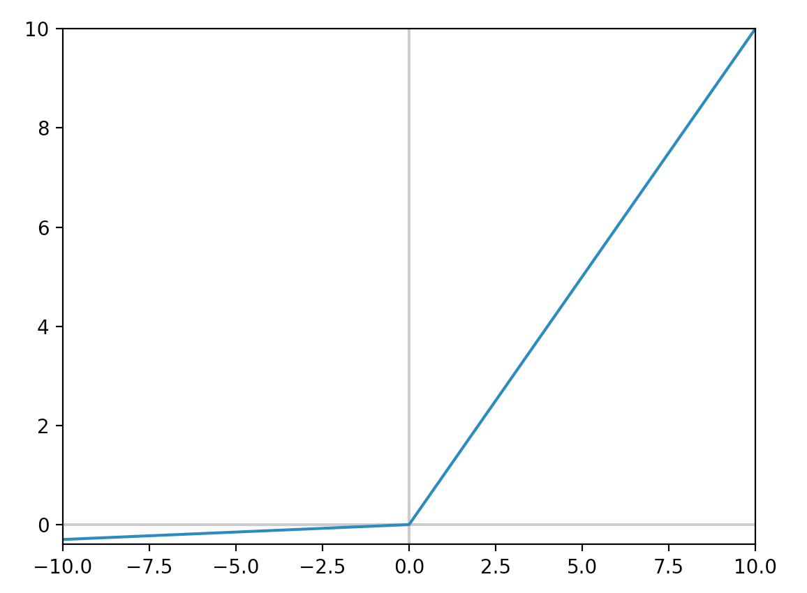
\(\alpha\) is a very small scalar value.
In general, we still use ReLU as an activation function with cares on the learning rate. However, if a large amount of node is dead, we should replace it with the leaky ReLU.
tanh
tanh is similar to sigmoid but the output is within [-1, 1] instead of [0, 1].
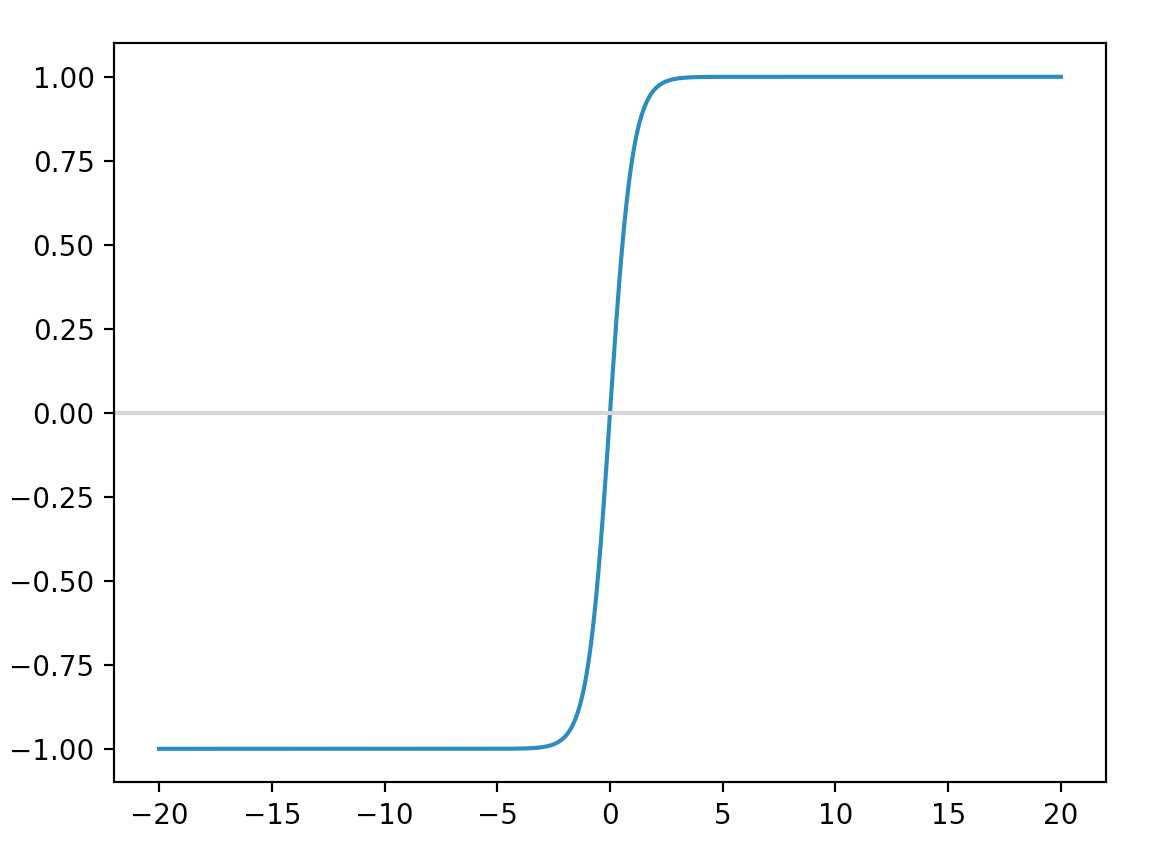
As mention before, we want the gradient descent to follow the curve of the cost function but not in some zip zap pattern. For the sigmoid function, the output value is always positive (between 0 and 1). The sign for the gradient relative to \(W\) subjects to the sign of \(x \frac {\partial J}{\partial l_{k+1}}\). Because \(x\) is always positive in a sigmoid output, the derivatives for this layer always follow the sign of \(\frac {\partial J}{\partial l_{k+1}}\).
\[\frac {\partial l_{k}}{\partial W} = x\frac {\partial J}{\partial l_{k+1}}\]So all \(W\) in this layer move in the same direction (all to the right or all to the left). The gradient descent will therefore follow a zip zap pattern instead. Since tanh has both positive and negative outputs, tanh does not have this problem as sigmoid.
Activation functions with NumPy
Numpy provides out of the box APIs to implement these functions.
import numpy as np
import matplotlib.pyplot as plt

def sigmoid(x):
  return 1 / (1 + np.exp(-x))

def relu(x):
  return np.maximum(0, x)

def tanh(x):
  return np.tanh(x)

x = np.arange(-20, 20, 0.001)

y = sigmoid(x)
plt.axvline(x=0, color="0.8")
plt.plot(x, y)
plt.show()

y = relu(x)
plt.axvline(x=0, color="0.8")
plt.axhline(y=0, color="0.8")
plt.plot(x, y)
plt.show()

y = tanh(x)
plt.plot(x, y)
plt.axhline(y=0, color="0.8")
plt.show()
Feed forward and backpropagation with sigmoid or ReLU
The derivative for the ReLU function is:
\[f(x)=\text{max}(0,x)\] \[\begin{equation} f'(x)= \begin{cases} 1, & \text{if}\ x>0 \\ 0, & \text{otherwise} \end{cases} \end{equation}\]The derivative for sigmoid is:
\[\sigma (x) = \frac{1}{1+e^{-x}}\]We can prove it with some calculus:
\[\begin{split} \frac{\partial \sigma(x)}{\partial x} & = \frac{1}{(1+e^{-x})^2} e^{-x} = \frac{1}{ (1+e^{-x})} \frac{1}{(1+e^{x})} \\ \\ &= \frac{1}{ (1+e^{-x})} (1 - \frac{1}{1+e^{-x}}) \\ \\ & = \sigma (x) (1-\sigma(x)) \\ \end{split}\]def relu_forward(x):
cache = x
out = np.maximum(0, x)
return out, cache
def relu_backward(dout, cache):
out = cache
dh = dout
dh[out < 0] = 0
return dh
def sigmoid_forward(x):
out = 1 / (1 + np.exp(-x))
return out, out
def sigmoid_backward(dout, cache):
dh = cache * (1-cache)
return dh * dout
Fully connected network
Let’s apply all our knowledge to build a fully connected network:
For each node in the hidden layer (except the last layer), we apply:
\[z_j = \sum_{i} W_{ij} x_{i} + b_{i}\] \[h(z_j)=\text{max}(0,z_{j})\]For the layer before the output, we apply only the linear equation but not the ReLU.
We will use 3 hidden layers.
z1, cache_z1 = affine_forward(X, W[0], b[0])
h1, cache_relu1 = relu_forward(z1)

z2, cache_z2 = affine_forward(h1, W[1], b[1])
h2, cache_relu2 = relu_forward(z2)

z3, cache_z3 = affine_forward(h2, W[2], b[2])
h3, cache_relu3 = relu_forward(z3)

z4, cache_z4 = affine_forward(h3, W[3], b[3])
Here is the corresponding backpropagation:
dz4, dW[3], db[3] = affine_backward(dout, cache_z4)

dh3 = relu_backward(dz4, cache_relu3)
dz3, dW[2], db[2] = affine_backward(dh3, cache_z3)

dh2 = relu_backward(dz3, cache_relu2)
dz2, dW[1], db[1] = affine_backward(dh2, cache_z2)

dh1 = relu_backward(dz2, cache_relu1)
_, dW[0], db[0] = affine_backward(dh1, cache_z1)
For those interested in details, we re-list some of the code below.
iteration = 100000
learning_rate = 1e-4
N = 100
...
def affine_forward(x, W, b):
    # x: input sample (N, D)
    # W: Weight (2, k)
    # b: bias (k,)
    # out: (N, k)
    out = x.dot(W) + b           # (N, D) * (D, k) -> (N, k)
    cache = (x, W, b)
    return out, cache

def affine_backward(dout, cache):
    # dout: dJ/dout (N, K)
    # x: input sample (N, D)
    # W: Weight (D, K)
    # b: bias (K, )
    x, W, b = cache

    if len(dout.shape)==1:
        dout = dout[:, np.newaxis]
    if len(W.shape) == 1:
        W = W[:, np.newaxis]

    W = W.T
    dx = dout.dot(W)

    dW = x.T.dot(dout)
    db = np.sum(dout, axis=0)

    return dx, dW, db

def relu_forward(x):
    cache = x
    out = np.maximum(0, x)
    return out, cache

def relu_backward(dout, cache):
    out = cache
    dh = dout
    dh[out < 0] = 0
    return dh

def mean_square_loss(h, y):
    # h: prediction (N,)
    # y: true value (N,)
    N = X.shape[0]                        # Find the number of samples
    h = h.reshape(-1)
    loss = np.sum(np.square(h - y)) / N   # Compute the mean square error from its true value y
    nh = h.reshape(-1)
    dout = 2 * (nh-y) / N                  # Compute the partial derivative of J relative to out
    return loss, dout

def compute_loss(X, W, b, y=None, use_relu=True):
    z1, cache_z1 = affine_forward(X, W[0], b[0])
    h1, cache_relu1 = relu_forward(z1)

    z2, cache_z2 = affine_forward(h1, W[1], b[1])
    h2, cache_relu2 = relu_forward(z2)

    z3, cache_z3 = affine_forward(h2, W[2], b[2])
    h3, cache_relu3 = relu_forward(z3)

    z4, cache_z4 = affine_forward(h3, W[3], b[3])

    if y is None:
        return z4, None, None

    dW = [None] * 4
    db = [None] * 4
    loss, dout = mean_square_loss(z4, y)

    dz4, dW[3], db[3] = affine_backward(dout, cache_z4)

    dh3 = relu_backward(dz4, cache_relu3)
    dz3, dW[2], db[2] = affine_backward(dh3, cache_z3)

    dh2 = relu_backward(dz3, cache_relu2)
    dz2, dW[1], db[1] = affine_backward(dh2, cache_z2)

    dh1 = relu_backward(dz2, cache_relu1)
    _, dW[0], db[0] = affine_backward(dh1, cache_z1)

    return loss, dW, db
...

W = [None] * 4
b = [None] * 4

W[0] = np.array([[0.7, 0.05, 0.0, 0.2, 0.2], [0.3, 0.01, 0.01, 0.3, 0.2]])  # (2, K)
b[0] = np.array([0.8, 0.2, 1.0, 0.2, 0.1])

W[1] = np.array([[0.7, 0.05, 0.0, 0.2, 0.1], [0.3, 0.01, 0.01, 0.3, 0.1], [0.3, 0.01, 0.01, 0.3, 0.1], [0.07, 0.04, 0.01, 0.1, 0.1], [0.1, 0.1, 0.01, 0.02, 0.03]])  # (K, K)
b[1] = np.array([0.8, 0.2, 1.0, 0.2, 0.1])

W[2] = np.array([[0.7, 0.05, 0.0, 0.2, 0.1], [0.3, 0.01, 0.01, 0.3, 0.1], [0.3, 0.01, 0.01, 0.3, 0.1], [0.07, 0.04, 0.01, 0.1, 0.1], [0.1, 0.1, 0.01, 0.02, 0.03]])  # (K, K)
b[2] = np.array([0.8, 0.2, 1.0, 0.2, 0.1])

W[3] = np.array([[0.8], [0.5], [0.05], [0.05], [0.1]])                 # (K, 1)
b[3] = np.array([0.2])

X = np.concatenate((education[:, np.newaxis], income[:, np.newaxis]), axis=1) # (N, 2) N samples with 2 features

for i in range(iteration):
    loss, dW, db = compute_loss(X, W, b, Y)
    for j, (cdW, cdb) in enumerate(zip(dW, db)):
        W[j] -= learning_rate * cdW
        b[j] -= learning_rate * cdb
    if i%20000==0:
        print(f"iteration {i}: loss={loss:.4}")
We also generate some testing data to measure how well our model predicts.
TN = 100
test_education = np.full(TN, 22)
test_income = np.random.randint(TN, size=test_education.shape[0])
test_income = np.sort(test_income)

true_model_Y = true_y(test_education, test_income)
true_sample_Y = sample(test_education, test_income, verbose=False)
X = np.concatenate((test_education[:, np.newaxis], test_income[:, np.newaxis]), axis=1)

out, _, _ = compute_loss(X, W, b)
loss_model, _ = mean_square_loss(out, true_model_Y)
loss_sample, _ = mean_square_loss(out, true_sample_Y)

print(f"testing: loss (compare with Oracle)={loss_model:.6}")
print(f"testing: loss (compare with sample)={loss_sample:.4}")
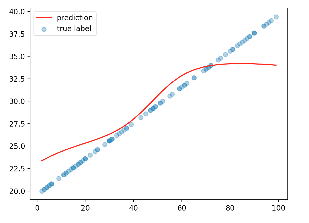
We plot the predicted values over the true values. The values derived from our Oracle model. For the first plot, we temporarily downsize the network to 1 hidden layers and fix the years of education to 22. We plot the number of dates with respect to income. The orange dots are our predictions. The blue dots are from the Oracle model after adding some random noise. The data match pretty well with each other.
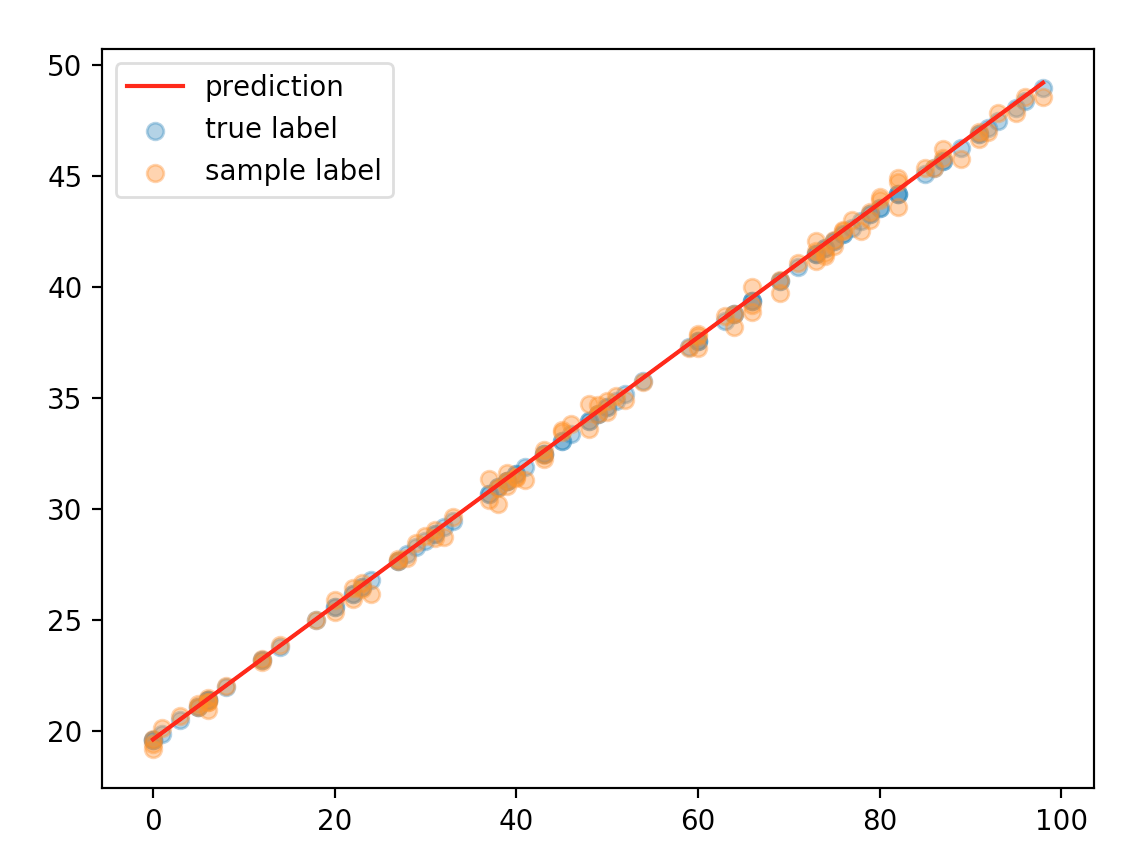
Congratulations! We just solved a problem using deep learning!
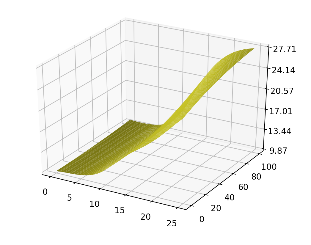
Now, we increase the number of hidden layers from 1 to 3. Do we improve the accuracy? In fact, our prediction’s accuracy drops. And the training requires more iterations and tuning.
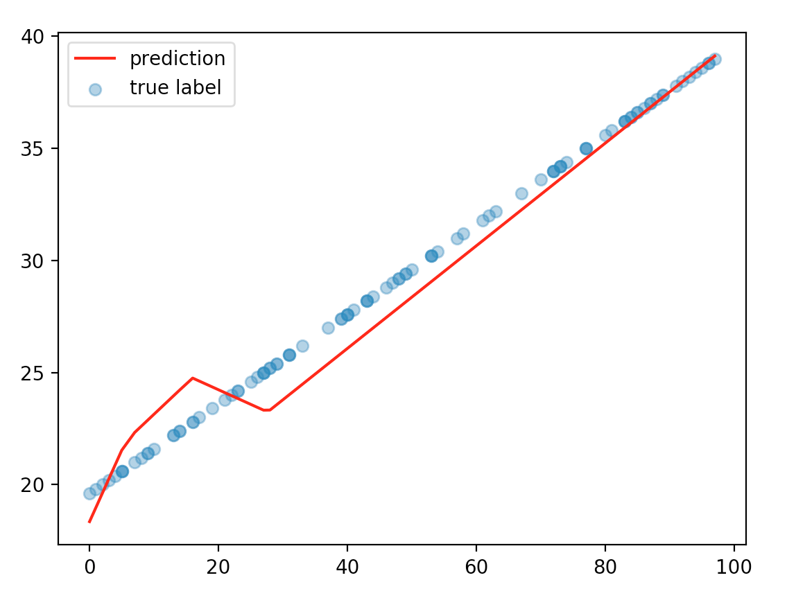
When we plot it in 3D with variable income and education, some part of the 2D plain is bent instead of flat.
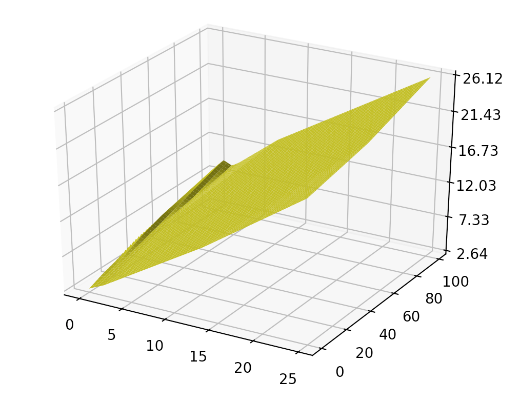
When we create the training dataset, we add some noise to our true value (# of dates). With a complex model, it increases its capability to model the noise also. If we have a large dataset, the effect of noise should cancel out. However, if the training dataset is not big enough, the accuracy suffers in comparison to the simpler model. As a general practice, we should start with a simple model and gradually increase its complexity. It is hard to start with a complex model when you have to deal with debugging and tuning at the same time.
def sample(education, income, verbose=True):
    dates = true_y(education, income)
    noise =  dates * 0.15 * np.random.randn(education.shape[0]) # Add some noise to our true model.
    return dates + noise
If you have limited training data, a complex model hurts the accuracy.
For completeness, we replace our ReLU function with a sigmoid function and plot the same diagram:
Here is the model we trained:
Layer 1:
      [[ 1.10727659,  0.22189273,  0.13302861,  0.2646622 ,  0.2835898 ],
       [ 0.23522207,  0.01791731, -0.01386124,  0.28925567,  0.187561  ]]

Layer 2:
 	[[ 0.9450821 ,  0.14869831,  0.07685842,  0.23896402,  0.15320876],
       [ 0.33076781,  0.02230716,  0.01925127,  0.30486342,  0.10669098],
       [ 0.18483084, -0.03456052, -0.01830806,  0.28216702,  0.07498301],
       [ 0.11560201,  0.05810744,  0.021574  ,  0.10670155,  0.11009798],
       [ 0.17446553,  0.12954657,  0.03042245,  0.03142454,  0.04630127]]),

Layer 3:
	[[ 0.79405847,  0.10679984,  0.00465651,  0.20686431,  0.11202472],
       [ 0.31141474,  0.01717969,  0.00995529,  0.30057041,  0.10141655],
       [ 0.13030365, -0.09887915,  0.0265004 ,  0.29536237,  0.07935725],
       [ 0.07790114,  0.04409276,  0.01333717,  0.10145275,  0.10112565],
       [ 0.12152267,  0.11339623,  0.00993313,  0.02115832,  0.03268988]]),

Layer 4:
	[[ 0.67123192],
       [ 0.48754364],
       [-0.2018187 ],
       [-0.03501616],
       [ 0.07363663]])]
Because we start with a random guess of \(W\), we can end up with models with different \(W\) for each run.
In the first part of the tutorial, we finish a simple FC network. We play with it to gain better insight. Almost the same code and techniques can be applied for real life problems. Nevertheless, training a deep network is not simple. In the second part of the tutorial, we cover those issues and find the corresponding resolutions. We will put things together with two real life visual recognition problems.